Abstract
Two-photon calcium imaging enables functional analysis of neuronal circuits by inferring action potential (AP) occurrence ("spike trains") from cellular fluorescence signals. It remains unclear how experimental parameters such as signal-to-noise ratio (SNR) and acquisition rate affect spike inference and whether additional information about network structure can be extracted. Here we present a simulation framework for quantitatively assessing how well spike dynamics and network topology can be inferred from noisy calcium imaging data. For simulated AP-evoked calcium transients in neocortical pyramidal cells, we analyzed the quality of spike inference as a function of SNR and data acquisition rate using a recently introduced peeling algorithm. Given experimentally attainable values of SNR and acquisition rate, neural spike trains could be reconstructed accurately and with up to millisecond precision. We then applied statistical neuronal network models to explore how remaining uncertainties in spike inference affect estimates of network connectivity and topological features of network organization. We define the experimental conditions suitable for inferring whether the network has a scale-free structure and determine how well hub neurons can be identified. Our findings provide a benchmark for future calcium imaging studies that aim to reliably infer neuronal network properties.
🔬 Techniques
✨ Fluorophores
🧪 Sample Preparation
💻 Software Details
🏛️ Research Organizations (ROR)
Affiliated research institutions:
📋 Methods
Simulation of single-neuron spike trains, calcium dynamics, and indicator fluorescence signals Simulation of single-neuron spike trains and calcium indicator fluorescence signals and all analysis were performed in Matlab (The Mathworks, Natick, MA, USA). We generated spike trains by a Poisson process assuming a low mean firing rate (0.2 Hz) similar to what has been reported for spontaneous activity of pyramidal cells in both anesthetized and awake rodent sensory cortex (Wolfe et al., 2010 ). In addition, to examine the effect of calcium indicator saturation we explored episodes of higher firing rates between 1 and 30 Hz as they occur in pyramidal neurons, e.g., upon sensory stimulation (Greenberg et al., 2008 ). A general description of AP-evoked fluorescence signals needs to consider the transformation of changes in intracellular free calcium concentration [Ca 2+ ] i to the particular type of fluorescence readout. Here, we use the widely adopted Δ F / F approach, expressing calcium signals as relative percentage fluorescence changes after background subtraction. In this case the transformation between [Ca 2+ ] i and fluorescence signal is given by (Helmchen, 2012 ): (1) [ Ca 2 + ] i = [ Ca 2 + ] rest + K d Δ F / F Δ F / F max ( 1 − Δ F / F Δ F / F max ) or reversely expressed by: (2) Δ F / F = Δ F / F max [ Ca 2 + ] i − [ Ca 2 + ] rest [ Ca 2 + ] i + K d Here, [Ca 2+ ] rest denotes the resting calcium concentration, K d the dissociation constant of the calcium indicator, and Δ F / F max the maximal Δ F / F reached upon saturation. Note that this transformation is a non-linear relationship. For fluorescence transients far from saturation ([Ca 2+ ] i « K d ) Equation 2 can be linearized to: (3) Δ F / F = Δ F / F max K d ( [ Ca 2 + ] i − [ Ca 2 + ] rest ) = Δ F / F max K d Δ [ Ca 2 + ] i This linear description is a good approximation for AP-evoked fluorescence signals in the low firing regime measured for example with a high-affinity indicator such as OGB-1 (Grewe et al., 2010 ) (Figures 9A,B ). In this case each AP evokes a stereotype, elementary somatic calcium transient, which can be approximated with a rapidly rising and exponentially decaying function: (4) Δ F / F = A ( 1 − e − ( t − t 0 ) / τ on ) e − ( t − t 0 ) / τ off for t ≥ t 0 Here, t 0 denotes the time point of spike occurrence, τ on the onset rise time, τ off the decay time, and A an amplitude scale parameter. The peak amplitude A Peak of the single-AP evoked calcium transient is given by: (5) A peak = A τ off ( τ on τ on + τ off ) τ on τ off ( τ on + τ off ) − 1 For the calcium indicator OGB-1, typical values of these parameters for neocortical pyramidal neurons are τ on = 10 ms, A peak = 7% Δ F / F , τ off = 0.5–1 s (Grewe et al., 2010 ). For the low firing regime we used the canonical elementary Δ F / F transient (Equation 4) as impulse response function. Other more complex shapes of the elementary transient, for example a double-exponential decay (Grewe et al., 2010 ), could be easily incorporated into the simulation framework. Because of the linear approximation, we obtained the fluorescence traces for the entire duration of the simulations by convolving the simulated spike trains with this elementary Δ F / F transient. Figure 9 Validation of simulation framework with experimental data. (A) Simultaneous cell-attached recording and high-speed two-photon calcium imaging in mouse neocortex in vivo . Top trace: cell-attached recording, APs marked by red dots. Bottom trace: measured cellular Δ F / F calcium signal (black) as well as simulated Δ F / F traces (red) for the recorded spike train. Imaging data were acquired with OGB-1 at 490 Hz sampling rate (Grewe et al., 2010 ). Note that a non-saturating model with double-exponential decay was used in this case to generate the simulated trace. (B) Simultaneous cell-attached recording and two-photon calcium imaging using the genetically-encoded calcium indicator YC3.60 (Lütcke et al., 2010 ). Top trace: cell-attached recording, APs marked by red dots. Bottom trace: measured cellular calcium signal (black) as well as simulated Δ F / F traces (red) for the recorded spike train (sampling rate: 7.81 Hz; expressed as relative percentage change Δ R / R of the YFP/CFP fluorescence ratio). A non-saturating model with single-exponential decay was used to generate the simulated trace. (C) Noise Δ F / F trace during episode without AP, as confirmed by simultaneous cell-attached recording (data not shown). Sampling rate: 490 Hz. (D) Left: distribution of signal intensities for data shown in (C) . Gaussian fit in red ( r 2 = 0.98). Right: distribution of goodness-of-fit of Gaussian fits ( r 2 ) for pooled data set (96 s total recording time). (E) Mean normalized autocovariance (±SD) for pooled noise data set. Peak at 0 s lag clipped. At higher AP firing rates, [Ca 2+ ] i may reach levels sufficiently high to cause substantial saturation of the calcium indicator. We therefore incorporated the possibility to account for indicator saturation in our simulation framework. Assuming a non-cooperative calcium binding characteristics, the saturation level S (ranging from 0 to 1) is given by: (6) S = [ CaB ] [ B ] T = [ Ca 2 + ] i [ Ca 2 + ] i + K d = [ Ca 2 + ] rest + K d Δ F / F Δ F / F max [ Ca 2 + ] rest + K d Here, [B] T denotes the indicator concentration in the cell and the equation's right side was obtained by insertion of equation 1. Importantly, indicator saturation not only leads to a non-linear transformation between [Ca 2+ ] i and Δ F / F but also directly affects buffered [Ca 2+ ] i dynamics, an aspect that has been neglected in previous attempts to incorporate indicator saturation in spike inference algorithms (Vogelstein et al., 2009 ; Stetter et al., 2012 ). Differentiation of Equation 6 with respect to [Ca 2+ ] i yields the so-called Ca 2+ -binding ratio κ B (or “buffering capacity”) of the indicator, which decreases with increasing [Ca 2+ ] i levels near saturation: (7) κ B = [ B ] T ∂ S ∂ [ Ca 2 + ] i = ∂ [ CaB ] ∂ [ Ca 2 + ] i = [ B ] T K d ( [ Ca 2 + ] i + K d ) 2 Note that the Ca 2+ -binding ratio critically depends on the indicator's Ca 2+ -binding affinity and its total concentration. The effect of adding an exogenous Ca 2+ -buffer such as the indicator on AP-evoked somatic calcium signals is well-understood for neocortical pyramidal neurons and is typically approximated by a single-compartment model, which assumes chemical equilibrium and neglects diffusion (Helmchen and Tank, 2011 ). The model additionally considers an endogenous Ca 2+ -binding ratio κ S , which we assumed to be constant [κ S = 100; (Helmchen et al., 1996 )], and the Ca 2+ extrusion rate γ (800 s −1 ) (Helmchen and Tank, 2011 ). [Ca 2+ ] rest was assumed 50 nM. The relaxation of [Ca 2+ ] i from an elevated level back to resting level is then described by the following non-linear differential equation: (8) d [ Ca 2 + ] i d t = − γ Δ [ Ca 2 + ] i ( 1 + κ S + κ B ) = − γ ( 1 + κ S + [ B ] T K d ( [ Ca 2 + ] i + K d ) 2 ) − 1 ( [ Ca 2 + ] i − [ Ca 2 + ] rest ) To calculate the model [Ca 2+ ] i traces for a given spike train, we numerically solved Equation 8 for each spike-to-spike interval starting from the [Ca 2+ ] i level reached after each AP. This level was calculated by incrementing the pre-AP [Ca 2+ ] i level at the moment of the next spike's occurrence t spike by (9) Δ [ Ca 2 + ] i ( t spike ) = Δ [ Ca 2 + ] T ( 1 + κ S + κ B ) = ( 1 + κ S + [ B ] T K d ( [ Ca 2 + ] i ( t spike ) + K d ) 2 ) − 1 Δ [ Ca 2 + ] T Here, Δ[Ca 2+ ] T denotes the total intracellular calcium concentration change caused by an AP, which was assumed 7.6 μM. The reduction of κ B at elevated [Ca 2+ ] i levels due to indicator saturation thus leads to an increase of Δ[Ca 2+ ] i per AP. The sharp increments of [Ca 2+ ] i for each spike were smoothed with an exponential rising onset function (τ on = 20 ms) similar to Equation 4. Finally, we transformed the [Ca 2+ ] i trace to a Δ F / F trace using equation 1, presuming the following reasonable parameter values for OGB-1: K d = 250 nM, [B] T = 50 μM, Δ F / F max = 93%. With these parameter settings, a single-AP evoked Δ F / F transient from resting [Ca 2+ ] i level was similar to the stereotype Δ F / F transient described by Equation 4. Note that despite the increased Δ[Ca 2+ ] i at elevated [Ca 2+ ] i levels the non-linear transformation between [Ca 2+ ] i and Δ F / F (Equation 1) has the effect that the Δ F / F -increment per AP becomes small closer to saturation (see Figure 4B ). For both the linear (low firing rate) and non-linear (higher firing rates) case, we added Gaussian white noise with standard deviation SD noise to the simulated Δ F / F traces. We assumed a realistic range of signal-to-noise ratios (SNR) for AP-evoked calcium transients, where we defined SNR as: (10) SNR = A peak S D noise We verified the assumption of Gaussian noise by empirically determining the noise distribution from random-access calcium imaging data (OGB-1; 490 Hz scan rate) (Grewe et al., 2010 ) when no spike had occurred (as verified by simultaneous electrophysiology). Without exception, noise distributions could be well-approximated by fitting a Gaussian curve ( r 2 = 0.96 ± 0.02), suggesting that residual noise in two-photon calcium imaging indeed can be assumed normally distributed (Figures 9C,D ) and contains little, if any, auto-correlation at lags >0.1 s (Figure 9E ). Gaussian noise is a reasonable assumption because the number of detected photons is likely to be much greater than 100 under two-photon imaging conditions (Ranganathan and Koester, 2010 ). We note that for extremely low light conditions this assumption may not be valid. As the last step in our generation of simulated Δ F / F traces, we subsampled the resulting noisy Δ F / F trace from the original temporal resolution of 2 kHz to a given target frame rate, f , by selecting the center data point for each time interval Δ t , where Δ t = 1/ f . In summary, our analysis indicates that the presented simulation framework provides a valid model for AP-evoked calcium signals measured in vivo using two-photon microscopy. While experimental data may be characterized by additional noise sources not captured in our model (for example slow drifts or motion artifacts), these are generally easy to identify and remove prior to further data analysis. Whereas the linear description is appropriate for many cases and has been widely adopted (Yaksi and Friedrich, 2006 ; Vogelstein et al., 2010 ; Mishchenko et al., 2011 ), we have here also generalized our approach to the non-linear regime by considering indicator saturation. Extension to include further non-linearities—such as for example saturation of endogenous buffers, cooperative indicator Ca 2+ -binding, e.g., for GECIs (Pologruto et al., 2004 ; Horikawa et al., 2010 ; Chen et al., 2013b ), or diffusional equilibration—will be straight forward. Likewise, other non-linear relationships between [Ca 2+ ] i and fluorescence readouts different from Δ F / F , for example using ratiometric measurements, could also be considered.
Show full methods section
Simulation of single-neuron spike trains, calcium dynamics, and indicator fluorescence signals Simulation of single-neuron spike trains and calcium indicator fluorescence signals and all analysis were performed in Matlab (The Mathworks, Natick, MA, USA). We generated spike trains by a Poisson process assuming a low mean firing rate (0.2 Hz) similar to what has been reported for spontaneous activity of pyramidal cells in both anesthetized and awake rodent sensory cortex (Wolfe et al., 2010 ). In addition, to examine the effect of calcium indicator saturation we explored episodes of higher firing rates between 1 and 30 Hz as they occur in pyramidal neurons, e.g., upon sensory stimulation (Greenberg et al., 2008 ). A general description of AP-evoked fluorescence signals needs to consider the transformation of changes in intracellular free calcium concentration [Ca 2+ ] i to the particular type of fluorescence readout. Here, we use the widely adopted Δ F / F approach, expressing calcium signals as relative percentage fluorescence changes after background subtraction. In this case the transformation between [Ca 2+ ] i and fluorescence signal is given by (Helmchen, 2012 ): (1) [ Ca 2 + ] i = [ Ca 2 + ] rest + K d Δ F / F Δ F / F max ( 1 − Δ F / F Δ F / F max ) or reversely expressed by: (2) Δ F / F = Δ F / F max [ Ca 2 + ] i − [ Ca 2 + ] rest [ Ca 2 + ] i + K d Here, [Ca 2+ ] rest denotes the resting calcium concentration, K d the dissociation constant of the calcium indicator, and Δ F / F max the maximal Δ F / F reached upon saturation. Note that this transformation is a non-linear relationship. For fluorescence transients far from saturation ([Ca 2+ ] i « K d ) Equation 2 can be linearized to: (3) Δ F / F = Δ F / F max K d ( [ Ca 2 + ] i − [ Ca 2 + ] rest ) = Δ F / F max K d Δ [ Ca 2 + ] i This linear description is a good approximation for AP-evoked fluorescence signals in the low firing regime measured for example with a high-affinity indicator such as OGB-1 (Grewe et al., 2010 ) (Figures 9A,B ). In this case each AP evokes a stereotype, elementary somatic calcium transient, which can be approximated with a rapidly rising and exponentially decaying function: (4) Δ F / F = A ( 1 − e − ( t − t 0 ) / τ on ) e − ( t − t 0 ) / τ off for t ≥ t 0 Here, t 0 denotes the time point of spike occurrence, τ on the onset rise time, τ off the decay time, and A an amplitude scale parameter. The peak amplitude A Peak of the single-AP evoked calcium transient is given by: (5) A peak = A τ off ( τ on τ on + τ off ) τ on τ off ( τ on + τ off ) − 1 For the calcium indicator OGB-1, typical values of these parameters for neocortical pyramidal neurons are τ on = 10 ms, A peak = 7% Δ F / F , τ off = 0.5–1 s (Grewe et al., 2010 ). For the low firing regime we used the canonical elementary Δ F / F transient (Equation 4) as impulse response function. Other more complex shapes of the elementary transient, for example a double-exponential decay (Grewe et al., 2010 ), could be easily incorporated into the simulation framework. Because of the linear approximation, we obtained the fluorescence traces for the entire duration of the simulations by convolving the simulated spike trains with this elementary Δ F / F transient. Figure 9 Validation of simulation framework with experimental data. (A) Simultaneous cell-attached recording and high-speed two-photon calcium imaging in mouse neocortex in vivo . Top trace: cell-attached recording, APs marked by red dots. Bottom trace: measured cellular Δ F / F calcium signal (black) as well as simulated Δ F / F traces (red) for the recorded spike train. Imaging data were acquired with OGB-1 at 490 Hz sampling rate (Grewe et al., 2010 ). Note that a non-saturating model with double-exponential decay was used in this case to generate the simulated trace. (B) Simultaneous cell-attached recording and two-photon calcium imaging using the genetically-encoded calcium indicator YC3.60 (Lütcke et al., 2010 ). Top trace: cell-attached recording, APs marked by red dots. Bottom trace: measured cellular calcium signal (black) as well as simulated Δ F / F traces (red) for the recorded spike train (sampling rate: 7.81 Hz; expressed as relative percentage change Δ R / R of the YFP/CFP fluorescence ratio). A non-saturating model with single-exponential decay was used to generate the simulated trace. (C) Noise Δ F / F trace during episode without AP, as confirmed by simultaneous cell-attached recording (data not shown). Sampling rate: 490 Hz. (D) Left: distribution of signal intensities for data shown in (C) . Gaussian fit in red ( r 2 = 0.98). Right: distribution of goodness-of-fit of Gaussian fits ( r 2 ) for pooled data set (96 s total recording time). (E) Mean normalized autocovariance (±SD) for pooled noise data set. Peak at 0 s lag clipped. At higher AP firing rates, [Ca 2+ ] i may reach levels sufficiently high to cause substantial saturation of the calcium indicator. We therefore incorporated the possibility to account for indicator saturation in our simulation framework. Assuming a non-cooperative calcium binding characteristics, the saturation level S (ranging from 0 to 1) is given by: (6) S = [ CaB ] [ B ] T = [ Ca 2 + ] i [ Ca 2 + ] i + K d = [ Ca 2 + ] rest + K d Δ F / F Δ F / F max [ Ca 2 + ] rest + K d Here, [B] T denotes the indicator concentration in the cell and the equation's right side was obtained by insertion of equation 1. Importantly, indicator saturation not only leads to a non-linear transformation between [Ca 2+ ] i and Δ F / F but also directly affects buffered [Ca 2+ ] i dynamics, an aspect that has been neglected in previous attempts to incorporate indicator saturation in spike inference algorithms (Vogelstein et al., 2009 ; Stetter et al., 2012 ). Differentiation of Equation 6 with respect to [Ca 2+ ] i yields the so-called Ca 2+ -binding ratio κ B (or “buffering capacity”) of the indicator, which decreases with increasing [Ca 2+ ] i levels near saturation: (7) κ B = [ B ] T ∂ S ∂ [ Ca 2 + ] i = ∂ [ CaB ] ∂ [ Ca 2 + ] i = [ B ] T K d ( [ Ca 2 + ] i + K d ) 2 Note that the Ca 2+ -binding ratio critically depends on the indicator's Ca 2+ -binding affinity and its total concentration. The effect of adding an exogenous Ca 2+ -buffer such as the indicator on AP-evoked somatic calcium signals is well-understood for neocortical pyramidal neurons and is typically approximated by a single-compartment model, which assumes chemical equilibrium and neglects diffusion (Helmchen and Tank, 2011 ). The model additionally considers an endogenous Ca 2+ -binding ratio κ S , which we assumed to be constant [κ S = 100; (Helmchen et al., 1996 )], and the Ca 2+ extrusion rate γ (800 s −1 ) (Helmchen and Tank, 2011 ). [Ca 2+ ] rest was assumed 50 nM. The relaxation of [Ca 2+ ] i from an elevated level back to resting level is then described by the following non-linear differential equation: (8) d [ Ca 2 + ] i d t = − γ Δ [ Ca 2 + ] i ( 1 + κ S + κ B ) = − γ ( 1 + κ S + [ B ] T K d ( [ Ca 2 + ] i + K d ) 2 ) − 1 ( [ Ca 2 + ] i − [ Ca 2 + ] rest ) To calculate the model [Ca 2+ ] i traces for a given spike train, we numerically solved Equation 8 for each spike-to-spike interval starting from the [Ca 2+ ] i level reached after each AP. This level was calculated by incrementing the pre-AP [Ca 2+ ] i level at the moment of the next spike's occurrence t spike by (9) Δ [ Ca 2 + ] i ( t spike ) = Δ [ Ca 2 + ] T ( 1 + κ S + κ B ) = ( 1 + κ S + [ B ] T K d ( [ Ca 2 + ] i ( t spike ) + K d ) 2 ) − 1 Δ [ Ca 2 + ] T Here, Δ[Ca 2+ ] T denotes the total intracellular calcium concentration change caused by an AP, which was assumed 7.6 μM. The reduction of κ B at elevated [Ca 2+ ] i levels due to indicator saturation thus leads to an increase of Δ[Ca 2+ ] i per AP. The sharp increments of [Ca 2+ ] i for each spike were smoothed with an exponential rising onset function (τ on = 20 ms) similar to Equation 4. Finally, we transformed the [Ca 2+ ] i trace to a Δ F / F trace using equation 1, presuming the following reasonable parameter values for OGB-1: K d = 250 nM, [B] T = 50 μM, Δ F / F max = 93%. With these parameter settings, a single-AP evoked Δ F / F transient from resting [Ca 2+ ] i level was similar to the stereotype Δ F / F transient described by Equation 4. Note that despite the increased Δ[Ca 2+ ] i at elevated [Ca 2+ ] i levels the non-linear transformation between [Ca 2+ ] i and Δ F / F (Equation 1) has the effect that the Δ F / F -increment per AP becomes small closer to saturation (see Figure 4B ). For both the linear (low firing rate) and non-linear (higher firing rates) case, we added Gaussian white noise with standard deviation SD noise to the simulated Δ F / F traces. We assumed a realistic range of signal-to-noise ratios (SNR) for AP-evoked calcium transients, where we defined SNR as: (10) SNR = A peak S D noise We verified the assumption of Gaussian noise by empirically determining the noise distribution from random-access calcium imaging data (OGB-1; 490 Hz scan rate) (Grewe et al., 2010 ) when no spike had occurred (as verified by simultaneous electrophysiology). Without exception, noise distributions could be well-approximated by fitting a Gaussian curve ( r 2 = 0.96 ± 0.02), suggesting that residual noise in two-photon calcium imaging indeed can be assumed normally distributed (Figures 9C,D ) and contains little, if any, auto-correlation at lags >0.1 s (Figure 9E ). Gaussian noise is a reasonable assumption because the number of detected photons is likely to be much greater than 100 under two-photon imaging conditions (Ranganathan and Koester, 2010 ). We note that for extremely low light conditions this assumption may not be valid. As the last step in our generation of simulated Δ F / F traces, we subsampled the resulting noisy Δ F / F trace from the original temporal resolution of 2 kHz to a given target frame rate, f , by selecting the center data point for each time interval Δ t , where Δ t = 1/ f . In summary, our analysis indicates that the presented simulation framework provides a valid model for AP-evoked calcium signals measured in vivo using two-photon microscopy. While experimental data may be characterized by additional noise sources not captured in our model (for example slow drifts or motion artifacts), these are generally easy to identify and remove prior to further data analysis. Whereas the linear description is appropriate for many cases and has been widely adopted (Yaksi and Friedrich, 2006 ; Vogelstein et al., 2010 ; Mishchenko et al., 2011 ), we have here also generalized our approach to the non-linear regime by considering indicator saturation. Extension to include further non-linearities—such as for example saturation of endogenous buffers, cooperative indicator Ca 2+ -binding, e.g., for GECIs (Pologruto et al., 2004 ; Horikawa et al., 2010 ; Chen et al., 2013b ), or diffusional equilibration—will be straight forward. Likewise, other non-linear relationships between [Ca 2+ ] i and fluorescence readouts different from Δ F / F , for example using ratiometric measurements, could also be considered.
Reconstruction of spike trains from calcium indicator signals
Action potentials were recovered from simulated Δ F / F traces using the peeling algorithm that we have introduced previously (Grewe et al., 2010 ). Briefly, AP-evoked fluorescence signal events were detected using Schmitt-trigger thresholding (high threshold: +1.75 SD, low threshold: −1 SD, minimal duration: 0.3 s) with additional integral check (at least 50% of theoretical noise-free integral). In the original peeling algorithm we assumed a linear relationship between [Ca 2+ ] i and Δ F / F , which we also applied here for the low firing regime. Specifically, a stereotype single-AP evoked Δ F / F transient waveform (with the same parameters as used for the simulation of [Ca 2+ ] i transients, unless noted otherwise) was iteratively subtracted (“peeled off”) as long as the integral of the residual trace remained positive and threshold-passing occurred. An advantage of the model-based nature of the peeling algorithm is that a non-linearity like indicator saturation can be easily incorporated. Here, we extended the peeling algorithm to take saturation into account, in order to enable spike reconstruction from saturating Δ F / F traces at high AP firing rates (up to 30 Hz). To this end, the single-AP evoked Δ F / F transient was re-calculated for each AP taking the respective pre-AP [Ca 2+ ] i level into account (again presuming parameter values for OGB-1; see above). More specific, the [Ca 2+ ] i -level dependent Δ F / F transient was calculated by taking the difference between the Δ F / F relaxation traces from post-AP and pre-AP levels (both computed by transforming the respective [Ca 2+ ] i decays, obtained by solving the differential Equation 8). For comparison of error rates we applied either the simple linear or the saturating peeling algorithm to [Ca 2+ ] i traces generated with a saturating indicator. For both the linear and saturating peeling approach, the temporal precision of detected spikes was further improved by optimization of spike times (±1 s around the spike time determined with the peeling algorithm; ±0.1 s for high AP rates). Optimization was performed by minimizing the squared sum of the residual trace using a pattern search algorithm (implemented in the Matlab Optimization toolbox). To examine spike detection performance independent of the particular Schmitt-trigger thresholds, we performed “precision-recall” (PR) analysis (see Table 1 ) by selecting combinations of Schmitt-trigger thresholds over wide ranges (high threshold: −2 to +5 SD; low threshold: −5 to +2 SD; minimal duration: 0–1 s) (Figures 2D,E ).
Within the framework of PR analysis
(Davis and Goadrich, 2006 ), we defined the break-even point as the data point closest to the unity line. Error rate α AP was defined as max(FDR, 1-TPR) at this point (range 0–1). Intuitively, α AP describes the distance of the break-even point from the upper-right corner of the PR-curve, which represents optimal performance (Davis and Goadrich, 2006 ). Table 1 Overview of spike metrics to quantify spike reconstruction accuracy . Simulated spikes may be either detected (true positive, TP) or missed (MS) by the reconstruction algorithm. We call the ratio of true discoveries to the total number of simulated spikes the True Positive Rate, TPR = TP/(TP + MS) or “recall.” On the other hand, spikes detected by the reconstruction algorithm may be matched by a simulated spike (true positive, TP) or represent false detections (false discovery, FD). We call the ratio of false discoveries to the total number of detected spikes the False Discovery Rate, FDR = FD/(TP + FD). In information retrieval theory (Davis and Goadrich, 2006 ), (1 − FDR) is also known as “precision.” Both TPR and FDR are defined as 0 for the special case of no simulated or reconstructed spikes, respectively. Comparison of original and reconstructed spike trains Spike time comparison was performed by successively matching spikes in the original and reconstructed spike train based on ascending spike time difference (up to a maximal difference of 0.5 s, see Figure 1D ). Remaining spikes in the original spike train reduce the true positive rate (calculated as fraction of total spikes in the original spike train) while spikes remaining in the reconstructed train contribute to the false discovery rate (calculated as a fraction of total spikes in the reconstructed spike train). We quantify reconstruction performance by the following parameters (Table 1 ): True positive rate (TPR): fraction of correctly detected spikes (out of total spikes in original spike train); TPR ∈ [0, 1], False discovery rate (FDR): fraction of false discoveries (out of total spikes in reconstructed spike train); FDR ∈ [0, 1], Temporal precision: mean and standard deviation of spike time differences between original and reconstructed spike trains, meanΔ t and σ Δ t , respectively (only for correct detections).
Large-scale network simulation and detailed neuron model
We simulated a network of 25,000 leaky integrate-and-fire neurons with conductance-based synapses (Zenke et al., 2013 ). 80% of the neurons were modeled as excitatory and 20% as inhibitory. Connectivity was chosen randomly with a density of 10%. In addition, each neuron received common excitatory input from a pool of 2000 independent Poisson processes that were connected randomly to all neurons with 10% probability. The rate of the external input was modeled as a pink noise stochastic process with a mean firing rate of 2 Hz per process and exhibiting fluctuations on all time scales (1/ f power spectrum) to mimick complex temporal dynamics of common-input in cortical networks. The network was tuned to the balanced state with asynchronous and irregular firing activity with a mean spiking activity of ~0.2 Hz. Specifically, the membrane voltage U i of a single cell i evolved according to: (11) τ m d U i d t = ( U rest − U i ) + g i exc ( t ) ( U exc − U i ) + g i inh ( t ) ( U inh − U i ) with membrane time constants τ m = 20 ms for excitatory neurons and τ m = 10 ms for inhibitory neurons, resting potential U rest =−70 mV, reversal potentials U exc = 0 mV and U inh = −80 mV and conductances g exc i ( t ) and g inh i ( t ) specified below. A spike was triggered when U i crossed the spiking threshold ϑ i . After each spike, U i was reset to the resting value U rest and the threshold ϑ i set to ϑ spike = 50 mV to implement a refractoriness mechanism. Following a reset, the threshold exponentially decayed to its resting value ϑ rest = −50 mV according to (12) τ thr d ϑ i d t = ( ϑ rest − ϑ i ) with time constant τ thr = 5 ms. The spike train S j ( t ) emitted by neuron j is given as S j ( t ) = ∑ k δ( t − t k j ), where the sum runs over all k corresponding spike times t k j . Inhibitory synaptic conductances of the downstream neurons were affected by presynaptic spikes as: (13) τ GABA d g i inh d t = − g i inh + ∑ j ∈ inh w i j S j ( t ) with τ GABA = 10 ms. Excitatory synapses were modeled containing a fast AMPA component with exponential decay (τ AMPA = 5 ms) and a slow NMDA component (τ NMDA = 100 ms): (14) τ AMPA d g i AMPA d t = − g i AMPA + ∑ j ∈ exc w i j S j ( t ) (15) τ NMDA d g i NMDA d t = − g i NMDA + g i AMPA The complete excitatory postsynaptic potential (EPSP) was obtained by a weighted sum of the AMPA and NMDA conductances: (16) g i exc ( t ) = 0.5 g i AMPA ( t ) + 0.5 g i NMDA ( t ) The weight values w ij of the synapse connecting neuron j with i ( w ij = 0 if the connection does not exist) are given as follows: w ( E → E ) = w ( E → I ) = 0.2 and w ( I → E ) = w ( I → I ) = 0.9. The external Poisson inputs were connected with a constant weight w (ext → E , I ) = 0.22. For computational efficiency, the voltage dependence of NMDA channels was omitted. All differential equations were integrated numerically using a forward Euler scheme with 0.1 ms time step using custom-written C/C++ code. Spike trains were generated for a total duration of T = 10,000 s.
Connectivity reconstruction based on coupled point process models
We selected subsets of N = 50 excitatory neurons from the population that had an average firing rate of 0.6 Hz or higher and reconstructed the connectivity between neurons of this subpopulation based on their spike trains of length T = 10,000 s. To extract the coupling, we fitted coupled GLMs to the spike trains. Full details on the methodology can be found in (Gerhard et al., 2011 ). Briefly, spike trains are discretized into a sequence of binary values which represent spiking activity within time windows of length 1 ms. The instantaneous firing probability for each time bin is modeled as a non-linear transformation of the sum of covariates. These include effects from past spiking of the neuron itself as well as spikes from other neurons. All coupling filters are parameterized using a set of spline basis functions and parameters are estimated using standard maximum-likelihood techniques. Note that the strength of the stochastic common-input to each neuron is unobserved and therefore not explicitly modeled. The coefficients corresponding to the cross-coupling filters are used to define the effective coupling structure: The integral of each interaction filter represents its strength (Gerhard et al., 2013 ). A binary decision about the presence of a directed link can be enforced by thresholding the matrix of coupling strengths. The pair of TPR links (fraction of correctly identified connections) and FDR links (false discovery rate) defines the error rate for the link reconstruction as the smallest α links that guarantees FDR links ≤ α links and TPR links ≥ 1−α links . Results generally show the averaged performance derived from the analysis of several random subpopulations of the full network. To derive the expected error rate in the link reconstruction under the assumption that the effect of the absolute detection power (α AP ) and spike time jitter (σ Δ t ) act independently (Figure 6F ), we use the intuition that detection powers ~1 − α would combine multiplicatively, so that, approximately: (17) α links , independent ≈ 1 − ( 1 − α links , due to α AP ) ( 1 − α links , due to σ Δ t ) 1 − α links ∗ where α * links is the best achievable error rate (in case of perfect spike reconstruction).
Cross-correlation analysis
For comparison, we also implemented a connectivity extraction algorithm based on spike count correlations. We binned the spike trains into bins of size Δ t cc and calculated the pairwise Pearson's cross-correlation coefficient of the resulting time series for each pair of neurons in the selected subpopulation. The negative logarithm of the significance value, i.e., the surprise, served as coupling strength. Note that this yielded symmetric (i.e., bidirectional) couplings. We swept through a wide range of values for Δt cc (0.5–500 ms) and chose the one with best performance, resulting in Δ t cc = 5 ms.
Surrogate model of spike train reconstruction
We perturbed the spike trains using surrogate transformations to simulate the effect of the errors introduced by imperfect spike reconstruction from noisy calcium imaging data. Specifically, we used the two key parameters that were used to describe the performance of the single-neuron spike reconstruction (error rate α AP and spike jitter σ Δ t ). For any error rate α AP >0, spikes were randomly removed from the simulated spike trains to match the desired TPR AP . Simultaneously, spikes were added at random times up to the prescribed level of FDR AP . The temporal imprecision σ Δ t was introduced by an additional jitter to all spike times given by a Gaussian distribution around zero with standard deviation σ Δ t . We repeated the connectivity estimation based on the perturbed spike trains and measured the performance using the error rate α links whose value should be compared to the reference value achievable in the case of unperturbed original spike trains (assuming perfect spike time reconstruction).
Identification of graph topology Scale-free networks
We generated scale-free networks of size 1000 neurons by constructing unweighted, undirected graphs whose degree distributions follow a power law p ( x ) ~ x −μ above a minimal degree k = 20 with exponent μ = 3, using the standard configuration model (Molloy and Reed, 1995 ). k was chosen as to produce an average link density of 4%, unless otherwise noted. We simulated the joint effect of calcium dynamics, spike train reconstruction and connectivity extraction by assuming that links are reconstructed with an error rate α links . This surrogate keeps the overall link density approximately constant. We then obtained the degree distribution of the reconstructed network and fitted a power law on its tail where the minimal degree and exponent were obtained using maximum-likelihood methods (Clauset et al., 2009 ). We constrained the exponent μ to be between 1 and 9 which covers all empirically observed scale-free networks. A goodness-of-fit test was applied to each fit using a Monte Carlo version of the Kolmogorov–Smirnov test (Clauset et al., 2009 ). We repeated the process of generation, imperfect reconstruction and re-fitting 1000 times and reported the median of the estimated power-law coefficient together with its standard deviation. We concluded that an estimated degree distribution was inconsistent with a power-law shape whenever the median p -value of the fit was below 0.05, i.e., a p -value < 0.05 occurred in more than half of the cases. Histograms of degree distributions were obtained with logarithmically spaced bins and by pooling distributions across all simulations. Hub neurons We generated scale-free networks of size 1000 neurons and power-law exponent μ = 3 as described above. We classified hub neurons in these networks as the 100 neurons with the highest degrees. We then simulated an imperfect network reconstruction as before and estimated how well neurons can be classified to be hub neurons as follows: The hit rate specifies the fraction of original hub neurons that belong to the 100 neurons with highest degree in the reconstructed network. A random assignment would lead to a hit rate of 10% (chance level). All estimates are based on 1000 simulations of independent networks.
Conflict of interest statement
The authors declare that the research was conducted in the absence of any commercial or financial relationships that could be construed as a potential conflict of interest.
Supplementary material The Supplementary Material for this article can be found online at: http://www.frontiersin.org/journal/10.3389/fncir.2013.00201/abstract Click here for additional data file.
📊 Figures
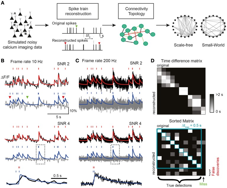
Figure 1
(A) Conceptual link between neuronal network dynamics and structure in our study. Network dynamics measurable with calcium imaging techniques is simulated to investigate how well spike trains can be r...
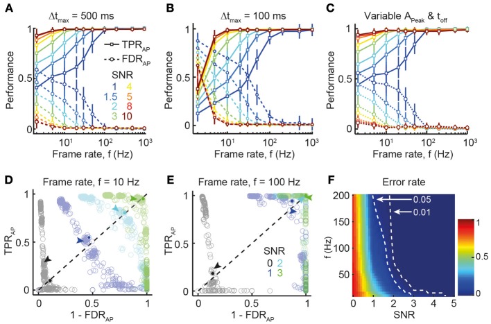
Figure 2
Dependence of spike reconstruction performance on SNR and frame rate. (A) TPR AP (solid lines) and FDR AP (dotted lines) as function of frame rate (x-axis) and SNR (different colors). Temporal window ...
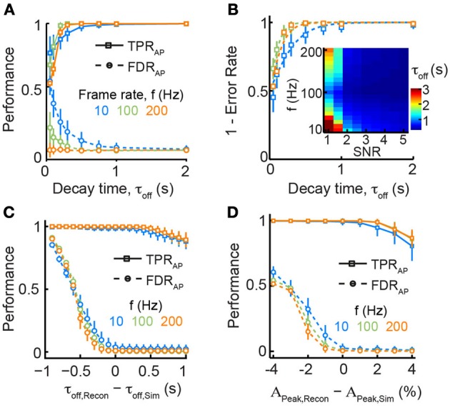
Figure 3
Dependence of spike train reconstruction on assumed calcium transient parameters. (A) TPR AP (solid lines) and FDR AP (dotted lines) as function of decay time u03c4 Off and frame rate f for fixed SNR ...
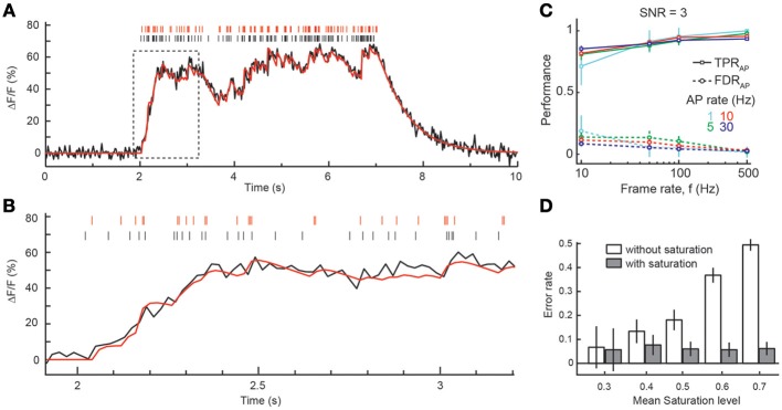
Figure 4
Spike inference from episodes with high firing rates. (A) Example simulation of an episode of 30 Hz firing for 5 s. The fluorescence trace was simulated with a frame rate of 50 Hz and SNR = 3 using th...
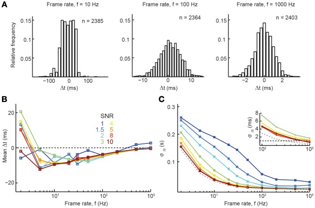
Figure 5
Precision of spike time inference. (A) Histogram of the spike time differences between original and reconstructed spike trains for 3 different frame rates ( SNR = 5). (B,C) Summary parameters for the ...
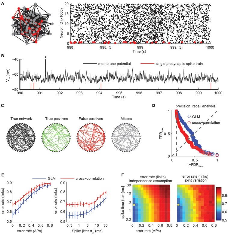
Figure 6
Connectivity extraction using imperfect spike trains. (A) A population of 25,000 excitatory and inhibitory neurons with sparse, random connectivity was simulated using integrate-and-fire models with c...
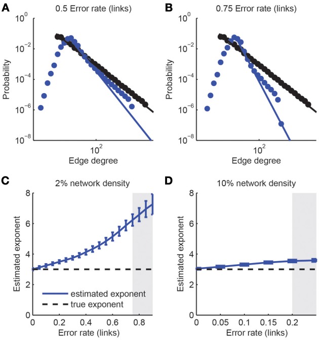
Figure 7
Detection of scale-free graphs upon imperfect connectivity reconstruction. (A,B) Degree distributions of networks after simulated reconstructions. The degree distribution of the original network (1000...
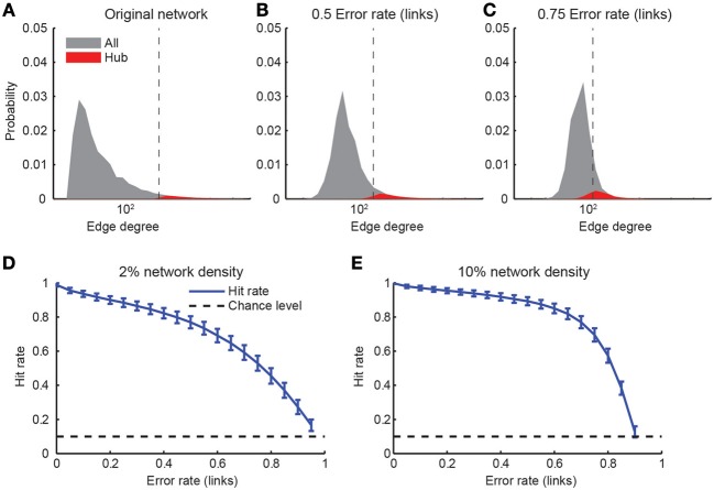
Figure 8
Detection of hub neurons upon imperfect connectivity reconstruction. (Au2013C) Degree distributions of networks after simulated reconstructions. The degree distribution of the original network (A) fol...
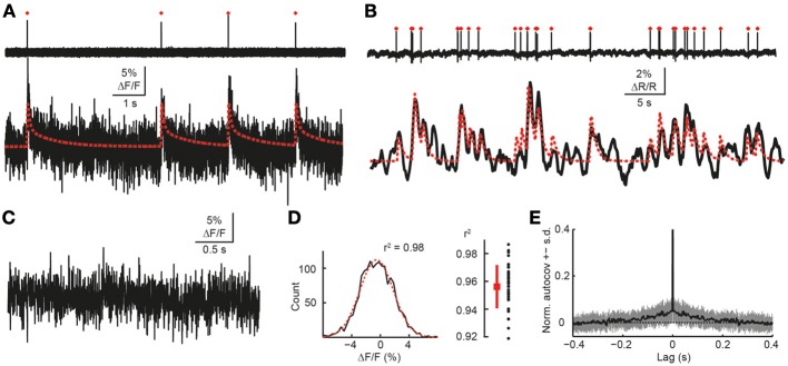
Figure 9
Validation of simulation framework with experimental data. (A) Simultaneous cell-attached recording and high-speed two-photon calcium imaging in mouse neocortex in vivo . Top trace: cell-attached reco...
Figure images are served from the NIH/NLM PubMed Central Open Access Subset or Europe PMC; copyright remains with the publishers and authors.
💬 Discussion
0 commentsNo comments yet. Be the first to start a discussion!
Leave a Comment