Abstract
Cellular microscopy images contain rich insights about biology. To extract this information, researchers use features, or measurements of the patterns of interest in the images. Here, we introduce a convolutional neural network (CNN) to automatically design features for fluorescence microscopy. We use a self-supervised method to learn feature representations of single cells in microscopy images without labelled training data. We train CNNs on a simple task that leverages the inherent structure of microscopy images and controls for variation in cell morphology and imaging: given one cell from an image, the CNN is asked to predict the fluorescence pattern in a second different cell from the same image. We show that our method learns high-quality features that describe protein expression patterns in single cells both yeast and human microscopy datasets. Moreover, we demonstrate that our features are useful for exploratory biological analysis, by capturing high-resolution cellular components in a proteome-wide cluster analysis of human proteins, and by quantifying multi-localized proteins and single-cell variability. We believe paired cell inpainting is a generalizable method to obtain feature representations of single cells in multichannel microscopy images.
🔬 Techniques
🧬 Organisms
✨ Fluorophores
🔬 Cell Lines
💻 Software Details
💻 Code & Software
💾 Data Repositories
🏛️ Research Organizations (ROR)
Affiliated research institutions:
📋 Methods
Paired cell inpainting We would like to learn a representation for single cells in a collection of microscopy images, I . We define each image i as a collection of single cells, i = { c i ,1 … c i , n }. We note that the only constraint on i is that its single cells C i must be considered similar to each other, so i does not need to be strictly defined as a single digital image so long as this is satisfied; in our experiments, we consider an “image” i to be all fields of view corresponding to an experimental well. We define single cells to be image patches, so c ∈ R H × W × Z , where Z are the channels. We split the images by channel into c = ( x , y ), where x ∈ R H × W × Z 1 , y ∈ R H × W × Z 2 , and Z 1 , Z 2 , ⊆ Z . For this work, we assign to Z 1 channels corresponding to structural markers, or fluorescent tags designed to visualize structural components of the cell, where all cells in the collection of images have been labeled with the tag. We assign to Z 2 channels corresponding to proteins, or channels where the tagged biomolecule will vary from image to image. We define a source cell c s , which is associated with a target cell c t satisfying constraints that both cells are from the same image, c s ∈ i s , c t ∈ i t , i s = i t , and c s ≠ c t . Our goal is to train a neural network that will solve the prediction problem y t ^ = f ( x s , y s , x t ) ∀ c s , c t ∈ I , where y t ^ represents the predicted protein channels that vary between images. For this work, we train the network on the prediction problem by minimizing a standard pixel-wise mean-squared error loss between the predicted target protein y t ^ and the actual target protein y t : L ( y t ^ , y t ) = 1 h ∙ w ∑ h , w ( y t ^ h , w - y t h , w ) 2 As with other self-supervised methods, our pretext training task is only meant to develop the internal feature representation of the CNN. After training, y t ^ is discarded, and the CNN is used as a feature extractor. Importantly, while our pretext task predicts a label y t , we consider our overall method to be unsupervised, because these labels are defined automatically from image content without any human supervision. One limitation in our pretext task is that some protein localizations are not fully deterministic in respect to the structure of the cell and are therefore challenging to predict given the inputs we define. In these cases, we observe that the network produces smoothed predictions that we hypothesize are an averaged guess of the localization. We show an example in Fig 1C ; while the source protein is localized to the nucleus in a punctate pattern, the target protein is predicted as a smooth distribution throughout the nucleoplasm. However, as our inpainting task is a pretext and discarded after training, we are not concerned with outputting fully realistic images. The averaging effect is likely due to our choice of a mean squared loss function; should more realistic images be desired, different loss functions, such as adversarial losses [ 33 ], may produce better results.
Show full methods section
Paired cell inpainting We would like to learn a representation for single cells in a collection of microscopy images, I . We define each image i as a collection of single cells, i = { c i ,1 … c i , n }. We note that the only constraint on i is that its single cells C i must be considered similar to each other, so i does not need to be strictly defined as a single digital image so long as this is satisfied; in our experiments, we consider an “image” i to be all fields of view corresponding to an experimental well. We define single cells to be image patches, so c ∈ R H × W × Z , where Z are the channels. We split the images by channel into c = ( x , y ), where x ∈ R H × W × Z 1 , y ∈ R H × W × Z 2 , and Z 1 , Z 2 , ⊆ Z . For this work, we assign to Z 1 channels corresponding to structural markers, or fluorescent tags designed to visualize structural components of the cell, where all cells in the collection of images have been labeled with the tag. We assign to Z 2 channels corresponding to proteins, or channels where the tagged biomolecule will vary from image to image. We define a source cell c s , which is associated with a target cell c t satisfying constraints that both cells are from the same image, c s ∈ i s , c t ∈ i t , i s = i t , and c s ≠ c t . Our goal is to train a neural network that will solve the prediction problem y t ^ = f ( x s , y s , x t ) ∀ c s , c t ∈ I , where y t ^ represents the predicted protein channels that vary between images. For this work, we train the network on the prediction problem by minimizing a standard pixel-wise mean-squared error loss between the predicted target protein y t ^ and the actual target protein y t : L ( y t ^ , y t ) = 1 h ∙ w ∑ h , w ( y t ^ h , w - y t h , w ) 2 As with other self-supervised methods, our pretext training task is only meant to develop the internal feature representation of the CNN. After training, y t ^ is discarded, and the CNN is used as a feature extractor. Importantly, while our pretext task predicts a label y t , we consider our overall method to be unsupervised, because these labels are defined automatically from image content without any human supervision. One limitation in our pretext task is that some protein localizations are not fully deterministic in respect to the structure of the cell and are therefore challenging to predict given the inputs we define. In these cases, we observe that the network produces smoothed predictions that we hypothesize are an averaged guess of the localization. We show an example in Fig 1C ; while the source protein is localized to the nucleus in a punctate pattern, the target protein is predicted as a smooth distribution throughout the nucleoplasm. However, as our inpainting task is a pretext and discarded after training, we are not concerned with outputting fully realistic images. The averaging effect is likely due to our choice of a mean squared loss function; should more realistic images be desired, different loss functions, such as adversarial losses [ 33 ], may produce better results.
Architecture
As the goal of our training task is to obtain a CNN that can encode single cell image patches into feature representations, we construct independent encoders for ( x s , y s ) and for x t , which we call the “source cell encoder” and the “target marker encoder”, respectively. After training with our self-supervised task, we isolate the source cell encoder, and discard all other components of our model. This architecture allows us to obtain a feature representation of any single cell image patch independently without also having to input target cell markers. To obtain single cell features, we simply input a single cell image patch, and extract the output of an intermediate convolutional layer in the source cell encoder. We show a summary of our architecture in Fig 1C . Following other work in self-supervised learning [ 17 , 18 , 30 ], we use an AlexNet architecture for the source cell encoder, although we set all kernel sizes to 3 due to the smaller sizes of our image patches, and we add batch normalization after each convolutional layer. We use a smaller number of filters and fewer convolutional layers in the architecture of the target marker encoder; we use three convolutional layers, with 16, 32, and 32 filters, respectively. Finally, for the decoder, we reverse the AlexNet architecture. The goal of our training is to develop the learned features of our source cell encoder, which will later be used to extract single cell feature representations. If the network were to utilize bleed-through from the fluorescent marker channels to predict the target marker image, or overfit to the data and ‘memorize’ the target cell images, then the network would not need to learn to extract useful information from the source cell images. To rule out that our trained models were subject to these effects, we produced inpainting results from a trained model, where we paired source cells with target cells where there is a mismatch between source and target protein localization. Here, the model has seen both the source and target cells during training, but never the specific pair due to the structure of our training task, as the cells originate from different images. We qualitatively confirmed that our trained networks were capable of synthesizing realistic results agreeing with the protein localization of the source cell ( S1 Fig ), suggesting that our models are not trivially overfitting to the target marker images. Sampling pairs Because the training inputs to our self-supervised task consist of pairs of cells, the number of possible combinations is large, as each cell may be paired with one of many other cells. This property is analogous to data augmentation, increasing the number of unique training inputs to our network. To sample training inputs, for each epoch, we iterate through every single cell in our training dataset, set it as the source cell, and draw with uniform probability a target cell from the set of all valid possible target cells. Our pretext task relies on the assumption that protein expression in single cells from the same image is similar. This assumption is not always true: in the datasets used in this work, some proteins exhibit significant single cell variability in their protein abundance or localization [ 34 , 35 ]. These proteins may contribute noise because paired single cells will have (unpredictably) different protein expression patterns and the model will not learn. Although the Human Protein Atlas documents variable proteins [ 24 ], for our experiments we do not remove these and confirm that our model still learns good features in spite of this noise. Datasets, preprocessing, and training For yeast cells, we used the WT2 dataset from the CYCLoPS database [ 36 ]. This collection expresses a cytosolic red fluorescent protein (RFP) in all cells, and tags proteins of interest with green fluorescent protein (GFP). We use the RFP channel as the structural marker, and the GFP channel as the protein. To extract single cell crops from the images in this dataset, we segmented our images using YeastSpotter on the structural marker channel [ 37 ], and extract a 64x64 pixel crop around the identified cell centers; we discarded any single cells with an area smaller than 5% or greater than 95% of the image crop, as these are likely artifacts arising from under- or over-segmentation. We discard any images with fewer than 30 cells. We preprocessed crops by rescaling each crop to be in the range of [0, 1]. These preprocessing operations result in a total of 1,165,713 single cell image patches grouped into 4,069 images (where each image is 4 fields of view), with a total of 4,069 of 4,138 proteins passing this filter. We also trained a second different yeast cell model, using a NOP1pr-GFP library previously published by Weill et al . [ 37 ] This collection tags all proteins of interest with GFP at the N-terminal of proteins with a NOP1 promoter, and is also imaged in brightfield. We used the brightfield channel as a structural marker and the GFP channel as the protein. We extracted and preprocessed single cell crops using the same procedure for the CYCLoPS dataset, and discarded any images with fewer than 30 single cells. These preprocessing operations result in a total of 563,075 single cell image patches grouped into 3,067 images (where each image is 3 fields of view), with a total of 3,067 of 3,916 proteins passing this filter. Finally, we trained a third yeast cell model, using a dataset previously published by Tkach et al . [ 38 ], a Nup49-RFP GFP-ORF library. This collection expresses a nuclear pore protein (Nup49) fused to RFP in all cells, and tags proteins of interest with green fluorescent protein (GFP). We use the RFP channel as the structural marker, and the GFP channel as the protein. We extracted and preprocessed single cell crops using the same procedure for the CYCLoPS dataset, and discarded any images with fewer than 30 single cells. These preprocessing operations result in a total of 1,733,127 single cell image patches grouped into 4,085 images (where each image is 3 fields of view), with a total of 4,085 of 4,149 proteins passing this filter. For human cells, we use images from version 18 of the Human Protein Atlas [ 24 ]. We were able to download jpeg images for a total of 12,068 proteins. Each protein may have multiple experiments, which image different cell line and antibody combinations. We consider an image to be of a protein for the same cell line and antibody combination; accordingly, we have 41,517 images (where each image is usually 2 fields of view). We downloaded 3 channels for these images. Two visualize the nuclei and microtubules, which we use as the structural marker channels. The third channel is an antibody for the protein of interest, which we use as the protein channel. To extract single cell crops from this image, we binarize the nuclear channel with an Otsu filter and find nuclei by labeling connected components as objects using the scikit-image package [ 39 ]. We filter any objects with an area of less than 400 pixels, and extract a 512x512 pixel crop around the center of mass of remaining objects. To reduce training time, we rescale the size of each crop to 64x64 pixels. We preprocessed crops by rescaling each crop to be in the range of [0, 1], and clipped pixels under 0.05 intensity for the microtubule and nuclei channels to 0 to improve contrast. Finally, we remove any images with fewer than 5 cells, leaving a total of 638,640 single cell image patches grouped into 41,285 images, with a total of 11,995 of 12,068 proteins passing this filter. Crop sizes for our datasets (64x64 pixels for yeast cells and 512x512 pixels for human cells) were chosen such that a crop fully encompasses an average cell from each of these datasets. We note that different image datasets may require different crop sizes, depending on the resolution of the images and the size of the cells. While each crop is centered around a segmentation, we did not filter crops with overlapping or clumped cells, so some crops may contain multiple cells. In general, we observed that our models did not have an issue learning to inpaint protein expression from a crop with multiple cells to a crop with a single cell, or vice versa: S1 Fig shows an example of a case where we inpaint protein expression from a crop with two cells to a crop with one cell. During training, we apply random horizontal and vertical flips to source and target cells independently as data augmentation. We trained models for 30 epochs using an Adam optimizer with an initial learning rate of 1e-4. After training, we extract representations by maximum pooling the output of an intermediate convolutional layer, across spatial dimensions. This strategy follows previous unsupervised representation extraction from self-supervised learning methods [ 17 , 30 ], which sample activations from feature maps.
Baseline feature extraction and benchmarking
To benchmark the performance of features learned using paired cell painting, we obtained features from other commonly-used feature representation strategies. As classic computer vision baselines for our yeast cell benchmarks, we obtained features extracted using CellProfiler [ 40 ] for a classification dataset of 30,889 image crops of yeast cells directly from the authors [ 41 ]. These features include measurements of intensity, shape, and texture, and have been optimized for classification performance. Further details are available from [ 41 ]. We also extracted features from these yeast cell image crops using interpretable expert-designed features by Handfield et al . [ 1 ] We followed procedures previously established by the authors: we segmented cells using provided software, and calculated features from the center cell in each crop. For our transfer learning baselines in our yeast cell benchmarks, we used a VGG16 model pretrained on ImageNet, using the Keras package. We benchmarked three different input strategies: (1) we mapped channels arbitrarily to RGB channels (RFP to red, GFP to green, blue channel left empty); (2) we inputted each channel separately as a greyscale image and concatenated the representations; (3) we inputted only the GFP channel as a greyscale image and used this representation alone. In addition, we benchmarked representations from each convolutional layer of VGG16, post-processed by maximum pooling across spatial dimensions (as we did for our self-supervised features). S2 Fig shows classification performance using each layer in VGG16 with the k NN classifier described in our benchmarks, across all three strategies. In general, we observed that the 3 rd input strategy resulted in superior performance, with performance peaking in the 4 th convolutional block of VGG16. We report results from the top-performing layer using the top-performing input strategy in our benchmarks. Contrary to previous work in transfer learning on microscopy images by Pawlowski et al ., we extract features from the intermediate convolutional layers of our transferred VGG16 model instead of the final fully-connected layer [ 15 ]. This modification allows us to input our images at their original size, instead of resizing them to the size of the images originally used to train the transferred model. As our work operates on single cell crops, which are much smaller than the full images benchmarked in previous work (64x64 pixels compared to 1280x1024 pixels), we found that inputting images at their original size instead of stretching them resulted in performance gains: our top-performing convolutional layer (block4_conv1) with inputs at original size achieved 69.33% accuracy, whereas resizing the images to 224x224 and using features from the final fully-connected layer (as-is, without max-pooling, as described in [ 15 ]) achieves 65.64% accuracy. In addition, we found that extracting features from images at original resolution improves run-time: on our machine, inputting 64x64 crops and extracting features from the best-performing layer was about 16 times faster than inputting resized 224x224 images and extracting features from the final fully-connected layer. Finally, for the supervised baseline, we used the model and pretrained weights provided by Kraus et al . [ 6 ]. We inputted images as previously described. To ensure that metrics reported for these features were comparable with the other accuracies we reported, we extracted features from this model and built the same classifier used for the other feature sets. We found that features from the final fully connected layer before the classification layer performed the best, and report results from this layer. To compare the performance of various feature representations with our single yeast cell dataset, we built k NN classifiers. We preprocessed each dataset by centering and scaling features by their mean and standard deviation. We employed leave-one-out cross-validation and predicted the label of each cell based on its neighbors using Euclidean distance. S1 Table shows classification accuracy with various parameterizations of k . We observed that regardless of k , feature representations were ranked the same in their classification performance, with our paired cell inpainting features always outperforming other unsupervised feature sets. However, k = 11 produced the best results for all feature sets, so we report results for this parameterization. As classic computer vision baselines for our human cell benchmarks, we curated a set of texture, correlation, and intensity features. For each crop, we measured the sum, mean, and standard deviation of intensity from pixels in the protein channels, and the Pearson correlation between the protein channel and the microtubule and nucleus channels. We extracted Haralick texture features from the protein channel at 5 scales (1, 2, 4, 8, and 16 pixels). Finally, as the transfer learning baseline for our human cell benchmarks, we extracted features from the pretrained VGG16 model using the same input strategies and layer as established in our yeast cell benchmark. Comparing pairwise distances in feature spaces To directly measure and compare how a feature set groups together cells with similar localizations in their feature spaces, measured the average pairwise distance between cells in the feature space. We preprocess single cell features by scaling to zero mean and unit variance, to control for feature-to-feature differences in scaling within feature sets. Then, to calculate the distance between two single cells c , we use the Euclidean distance between their features f : d ( c x , c y ) = ∥ f c x - f c y ∥ 2 . Given two images with the same localization term, we calculate the average distance of all cells in the first image paired with all cells in the second image and normalize these distances to an expectation of the average pairwise distance between images with different localization terms. A negative normalized average pairwise distance score indicates that the distances are smaller than expectation (so single cells in images with the same label are on average closer in the feature space). For the Human Protein Atlas images, we restricted our analysis to proteins that only had a single localization term shared by at least 30 proteins, resulting in proteins with 18 distinct localization terms (as listed in Fig 2B ). For each localization term, we calculated average pairwise distances for 1,000 random protein pairs with the same localization term, relative to an expectation from 1,000 random protein pairs with each of the possible other localization terms (for a total of 17,000 pairs sampled to control for class imbalance). For our experiments controlling for cell line, we also introduce the constraint that the images must be of cells of the same or different cell lines, depending on the experiment. Because some localization terms and cell line combinations are rare, we did not control for class imbalance and drew 10,000 random protein pairs with any different localization terms (not necessarily each other different term), and compared this to 10,000 random protein pairs with the same localization term. Hence, the distances in the two experiments are not directly comparable. 10.1371/journal.pcbi.1007348.g002 Fig 2 Quantitative comparisons of paired cell inpainting features with other unsupervised feature sets. (A) Overall and class-by-class performance benchmark for yeast single cell protein localization classes using unsupervised feature sets and a k NN classifier ( k = 11) on our test set. For all approaches extracting features from CNNs (Transfer Learning, Autoencoder, and Paired Cell Inpainting), we extract representations by maximum pooling across spatial dimensions, and report the top-performing layer. We report the overall accuracy as the balanced accuracy of all classes. (B) The normalized pairwise distance between cells with the same localization terms according to gene ontology labels, for proteins in the Human Protein Atlas. A more negative score indicates that cells are closer in the feature set compared to a random expectation. Single cell analysis of multiply-localized proteins For proteins localized to two compartments, we calculated a score for each cell based upon its distance to the first compartment versus its distance to the second compartment. To do so, we averaged the feature vectors for all single-cells in images annotated to localize to each compartment alone to define the average features for the two compartments. Then, for every single-cell, we calculated the distance of the single-cell’s features relative to the two compartments’ averages and take a log ratio of the distance to the first compartment divided by the distance to the second compartment. A negative number reflects that the single-cell is closer to the first compartment in the feature space, while a positive number reflects that the single-cell is closer to the second compartment.
Code availability
Code and pre-trained weights for the models used in this work are available at https://github.com/alexxijielu/paired_cell_inpainting .
Supporting information S1 Fig End-to-end paired cell inpainting results for pairs of cells unseen during training. We take four source human cells with different localizations (left-most boxes), belonging in the cytosol, nuclear membrane, nucleoli, and nucleoplasm, from top to bottom. For each of our source cells, we run our human cell model end-to-end with target markers from different images (left-center boxes) as input to generate predictions of the protein localization in these target cells (right-center boxes). We show the actual protein localization of the target cells (right-most boxes) to demonstrate that our model is capable of synthesizing results based on the source cells even when there is a mismatch between the source and target cell protein localization. (TIF) Click here for additional data file. S2 Fig Classification accuracies for representations extracted over each convolutional layer of a VGG16 model pretrained on ImageNet, for different input strategies. Images in the yeast single cell classification dataset were inputted using three different strategies: for “Concatenated”, we inputted the RFP and GFP channels independently as greyscale images and concatenated the representations; for “GFP-Only”, we inputted the GFP channel as a greyscale image and used this representation alone; and for “RGB Image”, we arbitrarily mapped channels to RGB channels (RFP to red, GFP to green, and blue left empty). Feature representations were extracted by maximum pooling the feature maps over spatial dimensions. We report the balanced classification accuracy using a leave-one-out kNN classifier ( k = 11) for these representations, identical to the one described in the “Paired cell inpainting features discriminate protein subcellular localization in yeast single cells” section of the Results. (TIF) Click here for additional data file. S3 Fig UMAP representations of various features, as labeled above each scatterplot, for our labeled single yeast cell benchmark dataset. All UMAPs are generated with the same parameters (Euclidean distance, 30 neighbors, minimum distance of 0.3). Embedded points are visualized as a scatterplot and are colored according to their label, as shown in the legend to the right. (TIF) Click here for additional data file. S4 Fig Averaged paired cell inpainting features for vesicle-only proteins in the Human Protein Atlas, using features from Conv3 of our human model trained on the Human Protein Atlas dataset, ordered using maximum likelihood agglomerative hierarchical clustering. We visualize features as a heat map, where positive values are colored yellow and negative values are colored blue, with the intensity of the color corresponding to magnitude. Columns in this heat map are features, while rows are proteins. Features have been mean-centered and normalized using all proteins in the dataset. We show three clusters (black and grey bars on the right), and crops of three representative images of the proteins within each of the clusters. For image crops, we show the protein channel in green, and the nucleus channel in blue. (TIF) Click here for additional data file. S5 Fig Averaged paired cell inpainting features from Conv4 of our yeast model trained on the NOP1pr-GFP dataset, for proteins labeled as punctuate in the NOP1pr-GFP library images, ordered using maximum likelihood agglomerative hierarchical clustering. We visualize features as a heat map, where positive values are colored yellow and negative values are colored blue, with the intensity of the color corresponding to magnitude. Columns in this heat map are features, while rows are proteins. Features have been mean-centered and normalized using all proteins in the dataset. We show three clusters (black and grey bars on the right), and crops of three representative images of the proteins within each of the clusters. For image crops, we show the protein channel only in green. For clusters B and C, we show the GO enrichment of the clusters relative to all punctate proteins; we list the q-value (the FDR-corrected p-value) and the number of proteins in the cluster with that annotation relative to the full size of the cluster. (TIF) Click here for additional data file.
S1 Table
Classification accuracies for feature sets with various parameterizations of k . Classification accuracies for single yeast cell localization classes using a k NN classifier on our test set of 30,889 labeled single cells, using various feature representations. We report the overall accuracy as the balanced accuracy of all classes. (DOCX) Click here for additional data file.
S2 Table
Classification accuracies for feature sets with logistic regression and random forest classifiers. Classification accuracies for single yeast cell localization classes using logistic regression and random forest classifiers on our dataset of 30,889 labeled single cells, built on various feature representations. We also report accuracy of the classifier end-to-end for the fully-supervised CNN in the last row of the table. Metrics are reported as the average balanced accuracy on the test sets under 5-fold cross-validation. We implemented all classifiers in Python using the scikit-learn package. For our logistic regression classifiers, we used a L1 penalty with a balanced class weight. For our random forest classifiers, we used 500 trees with 20% of the features used to determine best splits, and a balanced class weight. (DOCX) Click here for additional data file.
S1 Data
Full lists of the proteins in each cluster. (XLSX) Click here for additional data file.
S2 Data
Multi-localization scores for every cytosol-and-nucleoplasm and nucleoli-and-nucleus protein by cell line. (XLSX) Click here for additional data file.
📊 Figures

Fig 1
An overview of the inputs and targets to the network in paired cell inpainting, and of our proposed architecture.
(A) Inputs and targets to the network. We crop a source cell (green border) and a target cell (orange border) from the same image. Then, given all channels for the source cell, and the structural mark...
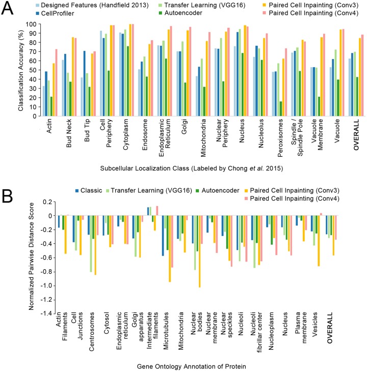
Fig 2
Quantitative comparisons of paired cell inpainting features with other unsupervised feature sets.
(A) Overall and class-by-class performance benchmark for yeast single cell protein localization classes using unsupervised feature sets and a k NN classifier ( k = 11) on our test set. For all approac...
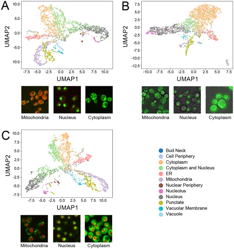
Fig 3
UMAP representations of protein-level paired cell inpainting representations for three independent yeast image datasets.
Protein-level representations are produced by averaging the features for all single cells for each protein. A) shows the CyCLOPS WT2 dataset, B) shows the dataset of Weill et al ., and C) shows the da...
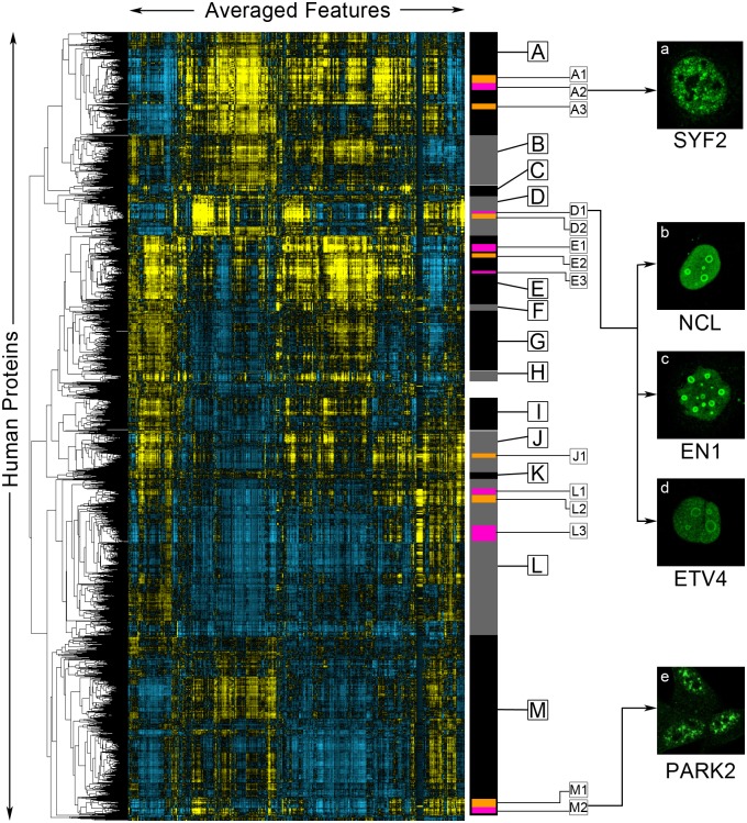
Fig 4
A clustered heat map of paired cell inpainting feature representation of proteins in the Human Protein Atlas.
Proteins are ordered using maximum likelihood agglomerative hierarchical clustering. We visualize the average of paired cell inpainting features for all cells for each protein as a heat map, where pos...
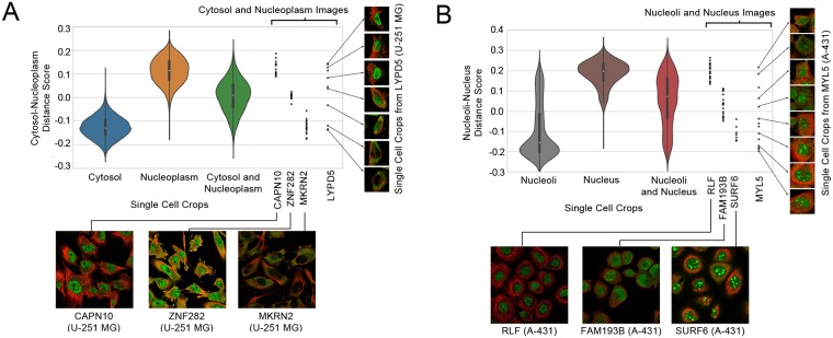
Fig 5
Single-cell scores (as explained in the text) for cytosolic-and-nucleoplasm cells (A), and nucleoli-and-nucleus cells (B).
We visualize single cells as violin plots. The black boxes inside the violin plots show the interquartile ranges and the white dots show the medians. To the right of the violin plots, we show all of t...
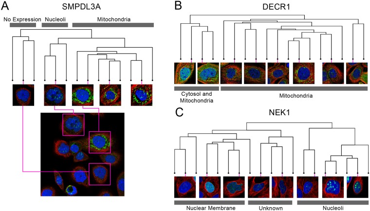
Fig 6
Dendograms from clustering the single-cell paired cell inpainting features of three spatially variable proteins: (A) SMPDL3A, (B) DECR1, (C) NEK1.
For each dendogram, we show single-cell image crops associated with representative branches of the dendogram. For (A) SMPDL3A, we also show a field of view of the image, and where various single-cell ...
Figure images are served from the NIH/NLM PubMed Central Open Access Subset or Europe PMC; copyright remains with the publishers and authors.
💬 Discussion
0 commentsNo comments yet. Be the first to start a discussion!
Leave a Comment