Abstract
SummaryElucidating the spatiotemporal organization of the genome inside the nucleus is imperative to our understanding of the regulation of genes and non‐coding sequences during development and environmental changes. Emerging techniques of chromatin imaging promise to bridge the long‐standing gap between sequencing studies, which reveal genomic information, and imaging studies that provide spatial and temporal information of defined genomic regions. Here, we demonstrate such an imaging technique based on two orthologues of the bacterial clustered regularly interspaced short palindromic repeats (CRISPR)–CRISPR associated protein 9 (Cas9). By fusing eGFP/mRuby2 to catalytically inactive versions of Streptococcus pyogenes and Staphylococcus aureus Cas9, we show robust visualization of telomere repeats in live leaf cells of Nicotiana benthamiana. By tracking the dynamics of telomeres visualized by CRISPR–dCas9, we reveal dynamic telomere movements of up to 2 μm over 30 min during interphase. Furthermore, we show that CRISPR–dCas9 can be combined with fluorescence‐labelled proteins to visualize DNA–protein interactions in vivo. By simultaneously using two dCas9 orthologues, we pave the way for the imaging of multiple genomic loci in live plants cells. CRISPR imaging bears the potential to significantly improve our understanding of the dynamics of chromosomes in live plant cells.
🔬 Techniques
🔭 Microscopes
🧬 Organisms
💻 Software
✨ Fluorophores
🧪 Sample Preparation
🏭 Microscope Brands
🧪 Reagent Suppliers
📷 Detectors
💻 Software Details
🏛️ Research Organizations (ROR)
Affiliated research institutions:
📋 Methods
T‐DNA construction All constructs are based on our previously described vector pCAS9‐TPC (Fauser et al ., 2014 ). For the two Cas9 orthologues from Streptococcus pyogenes (Sp) and Staphylococcus aureus (Sa), respective dCas9 versions were generated by two consecutive rounds of site‐directed mutagenesis, thereby introducing the two point mutations (D10A/H840A for Sp‐dCas9 and D10A/N580A for Sa‐dCas9). Plasmids encoding for eGFP (pSiM24‐eGFP) and mRuby2 (pcDNA3‐mRuby2) were obtained from Addgene ( http://www.addgene.com ). dCas9 and fluorescence protein (FP) sequences were generated with primers containing homologous flanks for subsequent Gibson Assembly cloning into the pCAS9‐TP backbone (for a full list of primers, see Appendix S8 ). The stop codons of the dCas9 and the first two FP sequences were removed to generate a continuous open reading frame (ORF), harbouring the respective dCas9 orthologue followed by a threefold fusion of the appropriate FP sequence. The dCas9 sequence and the FP fusion as well as the single FP sequences were linked via a GS‐rich linker, respectively. Protospacers were allowed to self‐anneal and the resulting 4‐bp overhangs were used for subsequent ligation into the respective pChimera vector via Bbs I restriction sites. The customised RNA chimeras were then ligated into the respective dCas9 vectors via Mlu I restriction sites. The Cas9 constructs developed in this study are available on request to HP.
Protospacer design
Protospacer sequences were selected based on the respective PAM sequence of each dCas9 orthologue, namely SpdCas9 and SadCas9, and synthesized as oligonucleotides with appropriate 4‐bp 5′ overhangs for cloning into the respective pChimera vector. The telomere‐specific protospacer (5′‐GGGTTTAGGGTTTAGGGTTT‐3′) is based on the Arabidopsis‐type telomere repeat sequence 5′‐(TTTAGGG)(n)‐3′. As a result of the presence of both Sp‐dCas9 (5′‐NGG‐3′) and Sa‐dCas9 (5′‐NNGRRT‐3′) PAM sequences in the telomere repeat sequence, both variants were used to label telomeres, which allowed us to compare these two orthologues. Transient transformation of N. benthamiana All CRISPR–dCas9 constructs, TRB1‐GFP (Schrumpfova et al ., 2014 ) and pUL50‐GFP (Lamm et al ., 2016 ) were separately transformed into Agrobacterium tumefaciens strain GV3101 by electroporation. Agrobacteria containing Sp‐dCas9, Sa‐dCas9 and pUL50‐GFP were cultured in YEB medium (5 g l ‐1 beef extract, 1 g l ‐1 yeast extract, 5 g l ‐1 peptone, 5 g l ‐1 sucrose, 300 mg l ‐1 MgSO4, 20 g l ‐1 agar) containing spectinomycin (100 μg ml −1 ) and rifampicin (50 μg ml −1 ). For TRB1‐GFP, Agrobacteria were cultured in YEB medium containing kanamycin (100 μg ml −1 ) and rifampicin (50 μg ml −1 ). The transient transformation of N. benthamiana leaf cells was performed as described in Phan and Conrad ( 2016 ). For the transformation of multiple constructs, bacterial cultures with an OD 600 between 1.0 and 1.3 were mixed in a 1:1 ratio prior to transformation. Plants were analysed 2–4 days after infiltration.
Show full methods section
T‐DNA construction All constructs are based on our previously described vector pCAS9‐TPC (Fauser et al ., 2014 ). For the two Cas9 orthologues from Streptococcus pyogenes (Sp) and Staphylococcus aureus (Sa), respective dCas9 versions were generated by two consecutive rounds of site‐directed mutagenesis, thereby introducing the two point mutations (D10A/H840A for Sp‐dCas9 and D10A/N580A for Sa‐dCas9). Plasmids encoding for eGFP (pSiM24‐eGFP) and mRuby2 (pcDNA3‐mRuby2) were obtained from Addgene ( http://www.addgene.com ). dCas9 and fluorescence protein (FP) sequences were generated with primers containing homologous flanks for subsequent Gibson Assembly cloning into the pCAS9‐TP backbone (for a full list of primers, see Appendix S8 ). The stop codons of the dCas9 and the first two FP sequences were removed to generate a continuous open reading frame (ORF), harbouring the respective dCas9 orthologue followed by a threefold fusion of the appropriate FP sequence. The dCas9 sequence and the FP fusion as well as the single FP sequences were linked via a GS‐rich linker, respectively. Protospacers were allowed to self‐anneal and the resulting 4‐bp overhangs were used for subsequent ligation into the respective pChimera vector via Bbs I restriction sites. The customised RNA chimeras were then ligated into the respective dCas9 vectors via Mlu I restriction sites. The Cas9 constructs developed in this study are available on request to HP.
Protospacer design
Protospacer sequences were selected based on the respective PAM sequence of each dCas9 orthologue, namely SpdCas9 and SadCas9, and synthesized as oligonucleotides with appropriate 4‐bp 5′ overhangs for cloning into the respective pChimera vector. The telomere‐specific protospacer (5′‐GGGTTTAGGGTTTAGGGTTT‐3′) is based on the Arabidopsis‐type telomere repeat sequence 5′‐(TTTAGGG)(n)‐3′. As a result of the presence of both Sp‐dCas9 (5′‐NGG‐3′) and Sa‐dCas9 (5′‐NNGRRT‐3′) PAM sequences in the telomere repeat sequence, both variants were used to label telomeres, which allowed us to compare these two orthologues. Transient transformation of N. benthamiana All CRISPR–dCas9 constructs, TRB1‐GFP (Schrumpfova et al ., 2014 ) and pUL50‐GFP (Lamm et al ., 2016 ) were separately transformed into Agrobacterium tumefaciens strain GV3101 by electroporation. Agrobacteria containing Sp‐dCas9, Sa‐dCas9 and pUL50‐GFP were cultured in YEB medium (5 g l ‐1 beef extract, 1 g l ‐1 yeast extract, 5 g l ‐1 peptone, 5 g l ‐1 sucrose, 300 mg l ‐1 MgSO4, 20 g l ‐1 agar) containing spectinomycin (100 μg ml −1 ) and rifampicin (50 μg ml −1 ). For TRB1‐GFP, Agrobacteria were cultured in YEB medium containing kanamycin (100 μg ml −1 ) and rifampicin (50 μg ml −1 ). The transient transformation of N. benthamiana leaf cells was performed as described in Phan and Conrad ( 2016 ). For the transformation of multiple constructs, bacterial cultures with an OD 600 between 1.0 and 1.3 were mixed in a 1:1 ratio prior to transformation. Plants were analysed 2–4 days after infiltration.
Immunofluorescence analysis and fluorescence in situ hybridization
Two or three days after leaf infiltration, nuclei were extracted by chopping a 1‐cm ² piece of leaf tissue in 1 ml of chromosome isolation buffer (Dolezel et al ., 2007 ) using a razor blade followed by filtration through a 35‐μm nylon mesh and subsequent centrifugation onto a microscopic slide at 400 rpm for 5 min (Shandon CytoSpin3, https://gmi-inc.com ). To confirm the specificity of each dCas9 construct, we conducted immunofluorescence staining against eGFP and mRuby2 in combination with fluorescence in situ hybridization (immuno‐FISH) against telomeres. Immuno‐FISH was performed as described by Ishii et al . ( 2015 ). eGFP was detected with a polyclonal GFP antibody (GFP antibody Dylight 488; Rockland, https://www.rockland-inc.com ) in a 1:2500 dilution. mRuby2 was detected with a primary RFP antibody [RFP antibody (5F8), 1:1000 dilution; Chromotek, http://www.chromotek.com ] generated in rats followed by an anti‐rat secondary antibody (ab96889; abcam, http://www.abcam.com ). To detect telomeres via FISH, we used 5′‐Cy5 labelled oligonucleotides composed of the same DNA sequence as the respective protospacer (sgRNA‐telomere, 5′‐GGGTTTAGGGTTTAGGGTTT‐3′). A final probe concentration of 0.33 μ m was used. The correct telomeric localization of our FISH probe was validated by testing on N. benthamiana chromosomes (Appendix S1 ) prepared from flower buds using a protocol described by Sanchez Moran et al . ( 2001 ).
Microscopic analyses
To analyse co‐localization between CRISPR–dCas9 imaging and FISH signals, images were acquired with an epifluorescence microscope (BX61; Olympus, https://www.olympus.com ) using a cooled charge coupled device (CCD) camera (Orca ER; Hamamatsu, http://www.hamamatsu.com ), and analysed with imagej . A total of 50 nuclei were analysed by immuno‐FISH to determine the efficiency of dCas9 to detect telomeres. The number of in vivo dCas9 signals was counted in 50 live nuclei to determine the in vivo labelling efficiency. To analyse the co‐localization of telomeres visualized by Sp‐dCas9 and TRB1, a total of 43 nuclei were analysed by epifluorescence microscopy.
Structured illumination microscopy
(SIM) was applied to a representative sample using a 63×/1.4Oil Plan‐Apochromat objective of an Elyra PS.1 microscope system with zen software (Carl Zeiss, https://www.zeiss.com ). Image stacks were captured separately for each fluorochrome using appropriate excitation and emission filters. Maximum intensity projections were generated from the stacks of SIM sections through the specimens in zen (3D rendering based on SIM image stacks was carried out using imaris 8.0; Bitplane, http://www.bitplane.com ). For live cell imaging of telomeres, fluorescence signals were analysed 2–4 days after infiltration with A. tumefaciens (see transient transformation of N. benthamiana ) by a LSM780 (Carl Zeiss). Infiltrated leaf areas were cut and mounted onto a microscopic slide. The distribution of fluorescence signals within the nucleus was recorded as z ‐stacks ( n = 50 nuclei). For a co‐distribution analysis, probes were excited with dual 488‐ and 561‐nm laser lines in combination with a 488/561‐nm beam splitter. eGFP emission was detected over a range of 490–540 nm, and mRuby2 emission was detected over a range of 570–620 nm. Photospectrometric analysis of the fluorescence signal by means of the META detector confirmed the identity of GFP and mRuby. The turnover of Sp‐dCas9‐eGFP telomeric signals was investigated by FRAP analysis. After two pre‐scans a region of interest of variable size was bleached. To achieve appropriate bleaching, the 488‐nm laser line was set at 100% power with 25 iterations at scan speed 7. Fluorescence intensity was followed over 30 min in 1‐min intervals.
Tracking of telomere signals and 3D image analysis
Telomere tracking based on time‐lapse z ‐stacks was conducted with imaris 8.0 (Bitplane). Brightness was manually adjusted to detect all telomere clusters. Tracking was performed using the autoregression motion algorithm, with a maximum distance of 20 μm and a maximum gap size of 3. Afterwards, the coordinates ( x , y , z ) of each spot at all time points were used to quantify telomere movements. Intertelomere distances were calculated for all telomeres of a representative nucleus based on differences in distance between time point 1 and time point 30. For this purpose, an intertelomere distance matrix was generated for time point 1 (matrix1) and time point 30 (matrix30). We then calculated the change in intertelomere distance by subtracting matrix1 from matrix30. The resulting matrix was then visualized as a heat map generated in rstudio using the heatmap 2 function of the gplots package. Distances are presented in μm and visualized by two different colours, indicating an increase (green) or decrease (red) of intertelomere distance over time. The 3D stacks of 12 live nuclei were semi‐automatically segmented and triangulated surfaces of nuclear boundaries were generated in amira 4.1 (Mercury Computer Systems, https://www.mrcy.com ). To account for relative nuclear movements (i.e. translations, rotations), 3D point clouds of telomere mass centres from subsequent time points ( t > 0) were rigidly registered to the reference system of coordinates given by the first time point ( t = 0) using absolute orientation quaternions (Horn, 1987 ). To characterize the intranuclear telomere motion, the MSD of telomeres relative to their initial position ( t = 0) was calculated as (1) MSD ( t ) = 1 N ∑ i = 1 N R i ( t ) − R i ( 0 ) 2 where R i ( t ) denotes the radius vector of the i ‐th registered telomere in the reference system of coordinates at time point t > 0. The intranuclear position of telomeres was quantified in three representative nuclei by the normalized radial distance (NRD): (2) NRD = TN / BN where TN and BN are the Euclidean distances between the nuclear envelope ( N ), the telomere ( T ) mass centres and the intersection point of the N–T line with the nuclear envelope surface ( B ), respectively. Accordingly, small NRD values indicate a nuclear‐central telomere location, whereas values close to 1 correspond to the nuclear periphery.
Supporting information Appendix S1. Telomere FISH on N. benthamiana chromosomes. Click here for additional data file. Appendix S2. Telomere FISH on N. benthamiana wild‐type interphase nucleus. Click here for additional data file. Appendix S3. Live interphase nucleus of N. benthamiana showing telomeres (Sp‐dCas9‐mRuby) and nuclear envelope (pUL50‐GFP). Click here for additional data file. Appendix S4. Dynamic imaging of telomeres by CRISPR–dCas9. Click here for additional data file. Appendix S5. 3D telomere localization. Click here for additional data file. Appendix S6. Telomere tracking. Click here for additional data file. Appendix S7. Registration of telomere movements to reference system. Click here for additional data file. Appendix S8. Primers used for T‐DNA construction. Click here for additional data file. Click here for additional data file.
📊 Figures
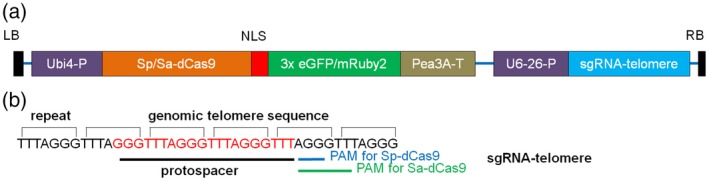
Figure 1
Structure of the CRISPR u2013 dC as9 construct. (a) Transcription of Sp/Sau2010 dC as9 was initiated by the parsley ubiquitin 4 promoter and terminated by the pea 3A terminator. An SV 40 NLS DNA seque...
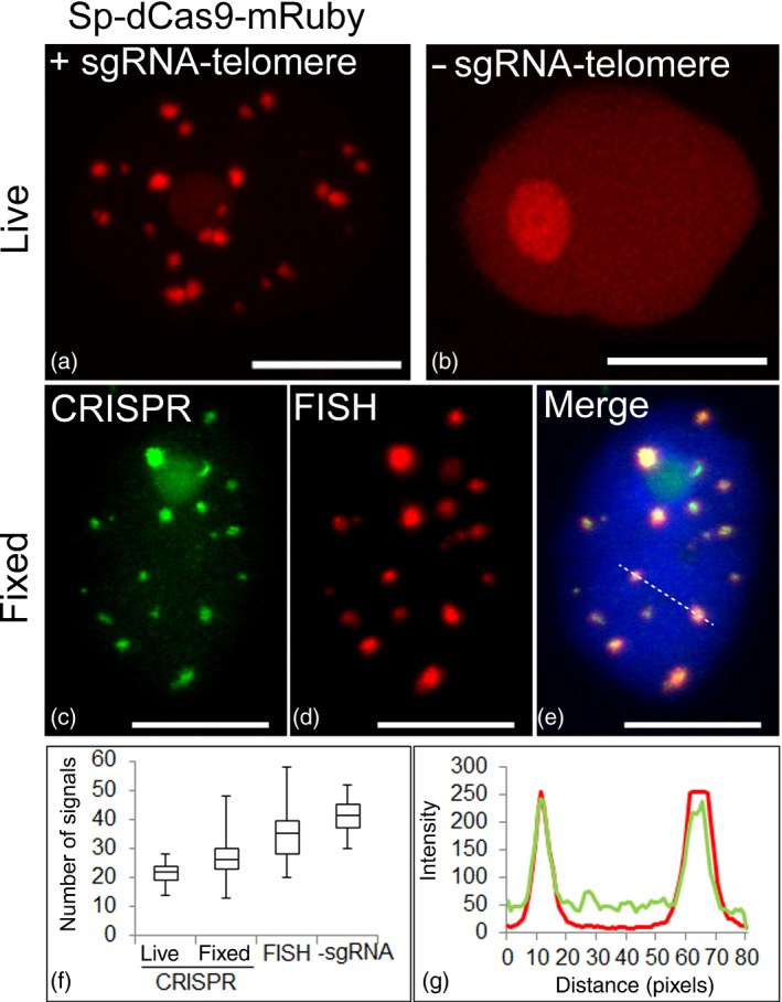
Figure 2
Live imaging of telomeres by CRISPR u2013 dC as9. (a) Spu2010 dC as9u2010mRuby and sg RNA u2010telomere were used for live imaging of telomeres in N. benthamiana leaf cells during interphase ( n =u00a...
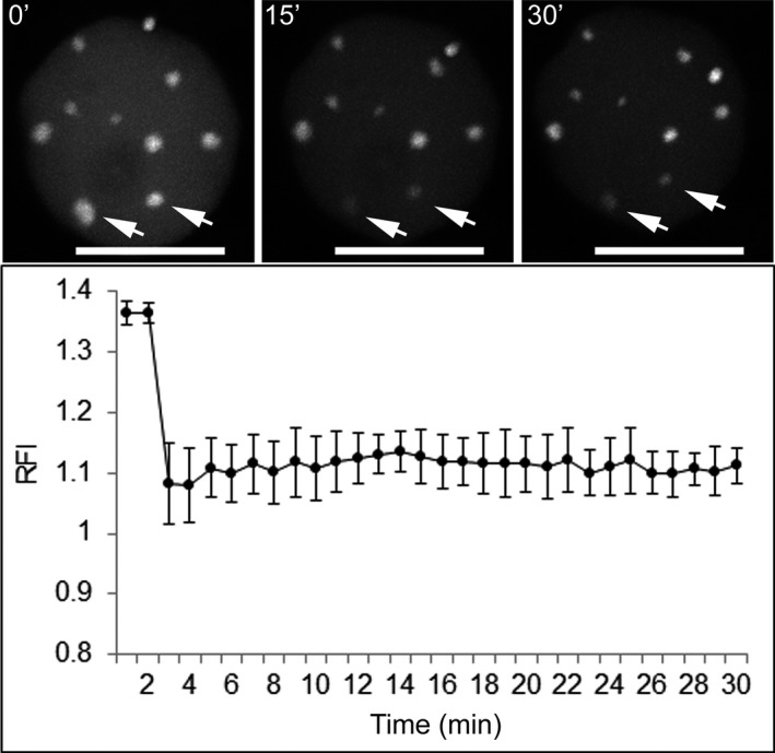
Figure 3
Fluorescence recovery after photobleaching ( FRAP ) analysis demonstrates a stable association of dC as9 with the target sequence during interphase. FRAP experiments were conducted on three individual...
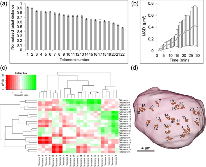
Figure 4
CRISPR u2013 dC as9 enables the 3D tracking of telomeres and reveals longu2010range movements in interphase nuclei. (a) Normalized radial distance ( NDR ) of telomeres of a representative nucleus. An ...
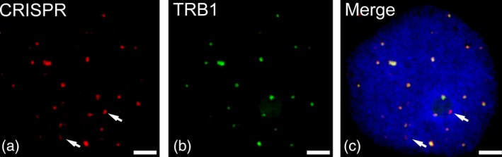
Figure 5
Simultaneous visualization of telomeric DNA by CRISPR u2013 dC as9 and the GFP u2010tagged telomeric repeat binding protein 1 ( TRB 1). (a) Immunofluorescence staining against Spu2010 dC as9u2010mRuby...
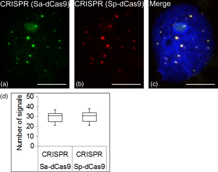
Figure 6
Comparison of Sau2010 dC as9 and Spu2010 dC as9. Telomeres were visualized by the simultaneous application of two dC as9 orthologues (Sau2010 dC as9 and Spu2010 dC as9). (a) Immunofluorescence stainin...
Figure images are served from the NIH/NLM PubMed Central Open Access Subset or Europe PMC; copyright remains with the publishers and authors.
💬 Discussion
0 commentsNo comments yet. Be the first to start a discussion!
Leave a Comment