Abstract
Luminal pH is an important functional feature of intracellular organelles. Acidification of the lumen of organelles such as endosomes, lysosomes, and the Golgi apparatus plays a critical role in fundamental cellular processes. As such, measurement of the luminal pH of these organelles has relevance to both basic research and translational research. At the same time, accurate measurement of intraorganellar pH in living cells can be challenging and may be a limiting hurdle for research in some areas. Here, we describe three powerful methods to measure rigorously the luminal pH of different intracellular organelles, focusing on endosomes, lysosomes, and the Golgi apparatus. The described methods are based on live imaging of pH-sensitive fluorescent probes and include: (1) A protocol based on quantitative, ratiometric measurement of endocytosis of pH-sensitive and pH-insensitive fluorescent conjugates of transferrin; (2) A protocol for the use of proteins tagged with a ratiometric variant of the pH-sensitive intrinsically fluorescent protein pHluorin; and (3) A protocol using the fluorescent dye LysoSensor™. We describe necessary reagents, key procedures, and methods and equipment for data acquisition and analysis. Examples of implementation of the protocols are provided for cultured cells derived from a cancer cell line and for primary cultures of mouse hippocampal neurons. In addition, we present strengths and weaknesses of the different described intraorganellar pH measurement methods. These protocols are likely to be of benefit to many researchers, from basic scientists to those conducting translational research with a focus on diseases in patient-derived cells.
🔬 Techniques
🔭 Microscopes
💻 Software
✨ Fluorophores
🧪 Sample Preparation
🔬 Cell Lines
🏭 Microscope Brands
🧪 Reagent Suppliers
💻 Software Details
🏛️ Research Organizations (ROR)
Affiliated research institutions:
📋 Methods
Materials and equipment Cell culture
To provide examples of implementation of the described protocols for measuring organellar pH, we have used: (1) a purchased line of cultured cells, namely, HAP1 cells (Horizon Discovery, Vienna, Austria) and (2) mouse primary hippocampal neurons dissected from post-natal day 0 (P0) to P1 mice. However, it is noted that the described methods can be applied to a wide variety of cell types. For HAP1 cell cultures, cells were grown in Iscove's Modified Dulbecco's Medium (IMDM) supplemented with 10% fetal bovine serum (FBS) and 1% penicillin–streptomycin. Cell cultures were maintained at 37°C in a humidified atmosphere of 95% air and 5% CO 2 . Cell culture medium and reagents used for HAP1 cells were obtained from ThermoFisher Scientific. For primary cultures of mouse hippocampal neurons, hippocampi were dissected from P0 to P1 mice, dissociated with papain (20 units/mL) in Earle's Balanced Salt Solution (EBSS) with bicarbonate at 37°C for 30 min, and triturated with a 1 mL pipette. Hippocampal neurons were plated on 35 mm glass bottom dishes (MatTek, Ashland, MA) pre-coated with 1 mg/mL poly-D-lysine at a cell density of 1.3 × 10 5 cells/mL in Neurobasal®-A medium supplemented with 2% B-27®, 1% GlutaMAX™, and 1% penicillin–streptomycin. Primary neuronal cultures were maintained at 37°C in a humidified atmosphere of 95% air and 5% CO 2 . Cell culture medium and reagents used for primary neuronal cultures were obtained from Worthington Biochemical Corporation (Lakewood, NJ). All experiments involving mice were carried out in accordance with the National Institutes of Health Guide for the Care and Use of Laboratory Animals (National Research Council of the National Academies, 2011 ). The protocol was approved by the Brown University Institutional Animal Care and Use Committee. pH calibration curve buffers For each protocol, a pH calibration curve needs to be generated in parallel with obtaining experimental data. Additionally, careful consideration should be given to ensuring that calibration curves obtained under similar conditions and using the same types of probes are consistent and exhibit a dynamic range appropriate for making accurate, reliable estimates of organellar pH 1 . For experiments for which results are provided herein, the pH calibration curve was generated as described previously (Xinhan et al., 2011 ; Ouyang et al., 2013 ) and as outlined below. The buffers for generating the pH calibration curve contain: 125 mM KCl, 25 mM NaCl, 10 μM monensin, and 25 mM N -[2-hydroxyethyl]-piperazine- N -[2-ethanesulfonic acid] (HEPES, pH 7.5 or 7.0) or 25 mM 2-[ N -morpholino] ethanesulfonic acid (MES, pH 6.5, 6.0, 5.5, 5.0, 4.5, 4.0, or 3.5). Each buffer solution is adjusted to the appropriate final pH using 1 N NaOH or 1 N HCl. See Table 1 for stock solutions and respective volumes for generating 50 mL aliquots of the pH calibration curve buffers. Table 1 Recipes for preparing pH calibration curve buffers. 1 M KCl 5 M NaCl 72 mM Monensin 0.5 M HEPES 0.5 M MES 1 N NaOH * 1 N HCl * H 2 O Buffer of pH 7.5 6.25 mL 0.25 mL 6.9 μL 2.5 mL – * * to 50 mL Buffer of pH 7.0 6.25 mL 0.25 mL 6.9 μL 2.5 mL – * * to 50 mL Buffer of pH 6.5 6.25 mL 0.25 mL 6.9 μL – 2.5 mL * * to 50 mL Buffer of pH 6.0 6.25 mL 0.25 mL 6.9 μL – 2.5 mL * * to 50 mL Buffer of pH 5.5 6.25 mL 0.25 mL 6.9 μL – 2.5 mL * * to 50 mL Buffer of pH 5.0 6.25 mL 0.25 mL 6.9 μL – 2.5 mL * * to 50 mL Buffer of pH 4.5 6.25 mL 0.25 mL 6.9 μL – 2.5 mL * * to 50 mL Buffer of pH 4.0 6.25 mL 0.25 mL 6.9 μL – 2.5 mL * * to 50 mL Buffer of pH 3.5 6.25 mL 0.25 mL 6.9 μL – 2.5 mL * * to 50 mL Final concentration 125 mM KCl 25 mM NaCl 10 μM Monensin 25 mM HEPES 25 mM MES – – – * Each buffer solution is adjusted to the appropriate final pH using 1 N NaOH or 1 N HCl .
Show full methods section
Materials and equipment Cell culture
To provide examples of implementation of the described protocols for measuring organellar pH, we have used: (1) a purchased line of cultured cells, namely, HAP1 cells (Horizon Discovery, Vienna, Austria) and (2) mouse primary hippocampal neurons dissected from post-natal day 0 (P0) to P1 mice. However, it is noted that the described methods can be applied to a wide variety of cell types. For HAP1 cell cultures, cells were grown in Iscove's Modified Dulbecco's Medium (IMDM) supplemented with 10% fetal bovine serum (FBS) and 1% penicillin–streptomycin. Cell cultures were maintained at 37°C in a humidified atmosphere of 95% air and 5% CO 2 . Cell culture medium and reagents used for HAP1 cells were obtained from ThermoFisher Scientific. For primary cultures of mouse hippocampal neurons, hippocampi were dissected from P0 to P1 mice, dissociated with papain (20 units/mL) in Earle's Balanced Salt Solution (EBSS) with bicarbonate at 37°C for 30 min, and triturated with a 1 mL pipette. Hippocampal neurons were plated on 35 mm glass bottom dishes (MatTek, Ashland, MA) pre-coated with 1 mg/mL poly-D-lysine at a cell density of 1.3 × 10 5 cells/mL in Neurobasal®-A medium supplemented with 2% B-27®, 1% GlutaMAX™, and 1% penicillin–streptomycin. Primary neuronal cultures were maintained at 37°C in a humidified atmosphere of 95% air and 5% CO 2 . Cell culture medium and reagents used for primary neuronal cultures were obtained from Worthington Biochemical Corporation (Lakewood, NJ). All experiments involving mice were carried out in accordance with the National Institutes of Health Guide for the Care and Use of Laboratory Animals (National Research Council of the National Academies, 2011 ). The protocol was approved by the Brown University Institutional Animal Care and Use Committee. pH calibration curve buffers For each protocol, a pH calibration curve needs to be generated in parallel with obtaining experimental data. Additionally, careful consideration should be given to ensuring that calibration curves obtained under similar conditions and using the same types of probes are consistent and exhibit a dynamic range appropriate for making accurate, reliable estimates of organellar pH 1 . For experiments for which results are provided herein, the pH calibration curve was generated as described previously (Xinhan et al., 2011 ; Ouyang et al., 2013 ) and as outlined below. The buffers for generating the pH calibration curve contain: 125 mM KCl, 25 mM NaCl, 10 μM monensin, and 25 mM N -[2-hydroxyethyl]-piperazine- N -[2-ethanesulfonic acid] (HEPES, pH 7.5 or 7.0) or 25 mM 2-[ N -morpholino] ethanesulfonic acid (MES, pH 6.5, 6.0, 5.5, 5.0, 4.5, 4.0, or 3.5). Each buffer solution is adjusted to the appropriate final pH using 1 N NaOH or 1 N HCl. See Table 1 for stock solutions and respective volumes for generating 50 mL aliquots of the pH calibration curve buffers. Table 1 Recipes for preparing pH calibration curve buffers. 1 M KCl 5 M NaCl 72 mM Monensin 0.5 M HEPES 0.5 M MES 1 N NaOH * 1 N HCl * H 2 O Buffer of pH 7.5 6.25 mL 0.25 mL 6.9 μL 2.5 mL – * * to 50 mL Buffer of pH 7.0 6.25 mL 0.25 mL 6.9 μL 2.5 mL – * * to 50 mL Buffer of pH 6.5 6.25 mL 0.25 mL 6.9 μL – 2.5 mL * * to 50 mL Buffer of pH 6.0 6.25 mL 0.25 mL 6.9 μL – 2.5 mL * * to 50 mL Buffer of pH 5.5 6.25 mL 0.25 mL 6.9 μL – 2.5 mL * * to 50 mL Buffer of pH 5.0 6.25 mL 0.25 mL 6.9 μL – 2.5 mL * * to 50 mL Buffer of pH 4.5 6.25 mL 0.25 mL 6.9 μL – 2.5 mL * * to 50 mL Buffer of pH 4.0 6.25 mL 0.25 mL 6.9 μL – 2.5 mL * * to 50 mL Buffer of pH 3.5 6.25 mL 0.25 mL 6.9 μL – 2.5 mL * * to 50 mL Final concentration 125 mM KCl 25 mM NaCl 10 μM Monensin 25 mM HEPES 25 mM MES – – – * Each buffer solution is adjusted to the appropriate final pH using 1 N NaOH or 1 N HCl .
Fluorescent transferrin conjugates Fluorescein isothiocyanate
(FITC)-conjugated transferrin (FITC-Tfn) and Alexa Fluor® 546-conjugated transferrin (Alexa Fluor® 546-Tfn) were from ThermoFisher Scientific. Of note, FITC-transferrin specifically needs to be used as opposed to Alexa Fluor® 488-transferrin, as FITC is pH-sensitive whereas Alexa Fluor® 488 is pH-stable across the pH range of interest. To this end, for the described protocol, FITC-Tfn acts as a pH sensor, whereas the Alexa Fluor® 546-Tfn acts as an internal standard for assessment of endocytic uptake and organellar localization. The reagent powders were diluted in Milli-Q H 2 O to stock solutions of 5 mg/mL, aliquoted, and stored at 4°C protected from light.
Plasmids for ratiometric phluorin-tagged proteins and cell transfection
Plasmids encoding for Golgi-localized proteins tagged with ratiometric pHluorin were provided by Terry E. Machen (University of California-Berkeley, Berkeley, CA) (Machen et al., 2003 ) and Yusuke Maeda (Osaka University, Suita, Osaka, Japan) (Maeda et al., 2008 ), the latter through an agreement with the Memorial Sloan Kettering Cancer Center (New York, NY). The plasmid encoding for transmembrane domains 1–3 of human Na + /H + exchanger 6 (NHE6) fused to pHluorin2 (hNHE6-TM1–3-pHluorin2), results for which are shown herein, was generated using the pHluorin2 vector (Mahon, 2011 ) and primers listed in Table S1 . The PCR products for NHE6 and pHluorin2 were digested using Bam HI restriction enzyme, ligated, and T-A cloned into pcDNA6.2-EmGFP/TOPO. The pcDNA6.2-EmGFP/TOPO vector was employed to take advantage of the CMV promotor; pHluorin2 has a stop codon, thus EmGFP will not be expressed. With respect to transfection of plasmids, for our studies we used either HAP1 cells or mouse primary hippocampal neurons and the transfection reagent Lipofectamine® 2000 (ThermoFisher Scientific). The manufacturer's protocol was followed, using a plasmid DNA to reagent ratio of 1:2. However, a variety of transfection reagents and methods exist, any of which might be acceptable so long as the method provides for a reasonable transfection efficiency in the chosen cell type. Steps for a typical transfection include. Passage cultured adherent cells the day before transfection; or plate primary cells a sufficient number of days in advance such that they are at the desired days in vitro (DIV) growth date at the time of transfection. Plate cells on 35 mm glass bottom dishes so as to achieve a confluency (for adherent cultured cells) of 70–90% at the time of transfection. As an example, this is estimated at 3 × 10 5 to 5 × 10 5 for HAP1 cells and at 1.3 × 10 5 for primary cultures of mouse hippocampal neurons. Transfect cells using the desired transfection reagent and method. Fluorescent dye LysoSensor™ LysoSensor™ Yellow/Blue DND-160 was from ThermoFisher Scientific. A 1 mM stock solution was prepared in anhydrous dimethyl sulfoxide (DMSO), aliquoted, and stored in the freezer (−5 to −30°C) protected from light. For cases in which fluorescence measurements were made using a microplate reader, a SpectraMax® M5 Microplate Reader equipped with SoftMax® Pro V5 software (Molecular Devices) was used. The 96 well cell culture microplates were from Greiner Bio-One (Kremsmünster, Austria). Confocal microscopy A Zeiss LSM 710 confocal laser scanning microscope and ZEN imaging software (ZEISS) were used for our studies. Additionally, during imaging, cells were maintained in a CO 2 chamber held at 37°C 2 . Cells were first located using a 10X or 20X objective. Upon identifying an appropriate field of view, images were then acquired using a 63X oil objective. For fluorescence image acquisition, laser and filter settings were adjusted according to the fluorescence excitation and emission requirements of the experimental setup and reagents (Table 2 ). Separate tracks were set to avoid signal crossing and the tracks were set to switch every line. Digital images were acquired at a frame size of 1,024 × 1,024 pixels. The master gain was set such that pixels were at maximal saturation without being oversaturated. Table 2 Peak excitation and emission wavelengths of reagents for measuring of intraorganellar pH. Reagent Excitation peak (nm) Emission peak (nm) Fluorescein isothiocyanate (FITC) 490 525 Alexa Fluor® 546 556 573 Ratiometric pHluorin 395 and 475 508 LysoSensor™ Yellow/Blue DND-160 329 and 384 440 and 540 Flow cytometry/fluorescence-activated cell sorting (FACS) For semi-adherent or non-adherent cells, flow cytometry can be used as an alternative to confocal microscopy for acquiring and analyzing data relating to ratiometric measurement of endocytosis of fluorescent conjugates of transferrin (Dunn and Maxfield, 2003 ). For our FACS-based analysis studies, we used the BD Influx™ cell sorter (BD Biosciences). We also used 5 mL polystyrene round-bottom tubes with cell-strainer caps and 5 mL polypropylene round-bottom tubes.
Software for data analysis
Fluorescence intensities were quantified using the software programs ImageJ (NIH) for confocal microscopy images, FlowJo™ (Ashland, OR) for FACS data, and SoftMax® Pro V5 (Molecular Devices) for data based on reading of microplates. Data were exported to a Microsoft Excel spreadsheet. The pH-values of organelles were determined by fitting data to the pH calibration curves generated concurrently with each set of experiments. Data are presented as the average ± standard error of the mean (SEM).
Stepwise procedures
Ratiometric measurement of fluorescent conjugates of transferrin This method takes advantage of a cell's endogenous endocytic pathway and the ubiquitous need for iron (Aisen and Listowsky, 1980 ; Sheftel et al., 2012 ). Endocytosis of transferrin, the iron-binding protein facilitating iron uptake in mammalian cells, and intracellular trafficking of the transferrin-transferrin receptor complex has long been studied. As such, the endocytic vesicle trafficking pathway of this ligand-receptor complex, namely, from early endosomes to recycling endosomes and back to the cell surface, is well known (Dautry-Varsat et al., 1983 ; Klausner et al., 1983 ; Maxfield and McGraw, 2004 ; Mayle et al., 2012 ). Furthermore, the pH of endocytic organelles involved in this trafficking has been determined for a variety of cell types, including through use of ratiometric fluorescence imaging or flow cytometry, with early studies performed in the 1980s and 1990s (Yamashiro et al., 1984 ; Sipe and Murphy, 1987 ; Sipe et al., 1991 ; Presley et al., 1993 ; Dunn et al., 1994 ). In the protocols described below, cells are incubated simultaneously with two different fluorescent conjugates—one pH-sensitive and the other pH-insensitive—of transferrin. The fluorescently labeled transferrin binds to its cognate transferrin receptor at the cell's plasma membrane. This binding event signals the endocytosis of the transferrin-transferrin receptor complex, which then, depending on the time frame allowed for transferrin loading and the cell type, is trafficked to early endosomes and recycling endosomes (Mayle et al., 2012 ; Reineke et al., 2015 ). Experimentally, the amount of time allowed for incubation with the fluorescent conjugates of transferrin affects which endosomal compartment(s) will be labeled. Here, based on the indicated incubation times, two related protocols for measuring the pH of early endosomes are provided, one for cases in which confocal microscopy is used as a means for acquiring data (i.e., adherent cells) and one for cases in which flow cytometry/FACS might be more appropriate as a means for acquiring data (i.e., semi-adherent/non-adherent cells).
Confocal microscopy-based protocol Generation of pH calibration curve Transferrin loading
One day before the experiment, passage cells and seed cells into a 35 mm glass bottom dish at a density of ~3 × 10 5 to ~5 × 10 5 . Alternatively, for primary cultures, plate cells a sufficient number of days in advance such that they are at the desired DIV growth date at the time of the experiment. On the day of the experiment, incubate cells in warm serum-free cell culture medium for 30 min at 37°C to remove any residual transferrin. Incubate cells for 30 min at 37°C in normal cell culture medium containing 66 μg/mL FITC-Tfn and 33 μg/mL Alexa Fluor® 546-Tfn (1 mL/dish). (See Table 3 for stock solutions and respective amounts for generating the indicated final concentrations of FITC-Tfn and Alexa Fluor® 546-Tfn in various volumes of cell culture medium.) Wash cells four times with 1X phosphate-buffered saline (PBS) and leave cells in 1 mL of 1X PBS. Table 3 Recipes for preparing FITC-Tfn and Alexa Fluor® 546-Tfn in cell culture medium. 5 mg/mL FITC-Tfn 5 mg/mL Alexa Fluor® 546-Tfn Cell culture medium 4.5 mL of medium 59.2 μL 30 μL to 4.5 mL 6.0 mL of medium 79 μL 40 μL to 6.0 mL 8.0 mL of medium 105.6 μL 52.8 μL to 8.0 mL Final concentration 66 μg/mL 33 μg/mL – Imaging Set the confocal microscope at excitation and emission filter settings appropriate for imaging of FITC and Alexa Fluor® 546 fluorophores (Table 2 ). Set separate tracks to avoid signal crossing and set the tracks to switch every line during image acquisition. Bring the dish of cells to the confocal microscope and find an appropriate region of cells for imaging using a low-power objective (e.g., 10X or 20X) and settings absent any activation of lasers (e.g., bright field) 2 . Rinse cells once with the most alkaline of the pH calibration curve buffers (e.g., pH 7.5). Incubate cells for 2 min in 1 mL of the first pH calibration curve buffer for imaging. Collect four images of cells using a high-power objective (e.g., 63X) relatively quickly and taking care not to shift the horizontal plane so as to help ensure that images do not get out of register. 3 Rinse cells once with 1X PBS and twice with the next pH calibration curve buffer in line, proceeding from most alkaline to most acidic. Incubate cells for 2 min in 1 mL of the pH calibration curve buffer used in step 6 for rinsing but now for imaging. Repeat steps 5–7 until images have been collected for cells incubated in at least five of the pH calibration curve buffers. Ensure to proceed from most alkaline (pH 7.5) to most acidic (pH 3.5).
Image analysis and plotting of data
For each pH calibration curve buffer, open the collected raw images (e.g., LSM, TIFF) in ImageJ. Select regions of interest within cells that are reflective of transferrin-labeled endosomal compartments and record the endosomal fluorescence intensity values. Additionally, select regions of interest outside of cells (i.e., background) and record the background fluorescence intensity values for each channel. For endosomal compartments, selection of regions of interest should be based on the Alexa Fluor® 546 signal; however, fluorescence intensity values should be recorded for both the FITC signal and Alexa Fluor® 546 signal. Export the fluorescence intensity measurement data to Microsoft Excel. Subtract the background fluorescence intensity values for each channel from the corresponding fluorescence intensity values relating to transferrin-labeled endosomes. Calculate the background-subtracted fluorescence intensity ratio of FITC signal:Alexa Fluor® 546 signal for each region of interest and for each pH calibration curve buffer. Calculate and plot the average FITC signal:Alexa Fluor® 546 signal ratio for each pH calibration curve buffer. Fit the data so as to generate a pH calibration curve for use in determining pH-values based on experimental data 1 .
Measurement of endosomal pH Transferrin loading
One day before the experiment, passage cells and seed cells into a 35 mm glass bottom dish at a density of ~3 × 10 5 to ~5 × 10 5 . Alternatively, for primary cultures, plate cells a sufficient number of days in advance such that they are at the desired DIV growth date at the time of the experiment. On the day of the experiment, incubate cells in warm serum-free cell culture medium for 30 min at 37°C to remove any residual transferrin. Incubate cells for 10 min at 37°C in normal cell culture medium containing 66 μg/mL FITC-Tfn and 33 μg/mL Alexa Fluor® 546-Tfn (1 mL/dish) (Table 3 ) 4 . Wash cells four times with 1X PBS. Incubate cells in 1 mL of phenol red-free cell culture medium. (Use of such cell culture medium is to reduce autofluorescence.)
Imaging
Set the confocal microscope settings to those used in collecting images to generate the pH calibration curve. Bring the dish of cells to the confocal microscope and find an appropriate region of cells for imaging 2 . Collect six to eight images of cells using a high-power objective (e.g., 63X) and the same settings as those used in collecting images to generate the pH calibration curve. Images should be acquired over a time span of not more than 7–8 min and taking care not to shift the horizontal plane so as to help ensure that images do not get out of register 3, 4 .
Image analysis and fitting of data
Open the collected raw images (e.g., LSM, TIFF) in ImageJ. Select regions of interest within cells that are reflective of transferrin-labeled endosomal compartments and record the endosomal fluorescence intensity values. Additionally, select regions of interest outside of cells (i.e., background) and record the background fluorescence intensity values for each channel. For endosomal compartments, selection of regions of interest should be based on the Alexa Fluor® 546 signal; however, fluorescence intensity values should be recorded for both the FITC signal and Alexa Fluor® 546 signal. Export the fluorescence intensity measurement data to Microsoft Excel. Subtract the background fluorescence intensity values for each channel from the corresponding fluorescence intensity values relating to transferrin-labeled endosomes. Calculate the background-subtracted fluorescence intensity ratio of FITC signal:Alexa Fluor® 546 signal for each region of interest (i.e., endosomes). Calculate the pH of each region of interest using the pH calibration curve generated in parallel with the experiment. Calculate the average pH for all measured regions of interest across all cells, thereby resulting in an average endosomal pH. Flow cytometry-based/FACS-based protocol Generation of pH calibration curve Transferrin loading One day before the experiment, passage cells and seed cells into a six well plate at a density of ~3 × 10 5 to ~5 × 10 5 . Alternatively, for primary cultures, plate cells a sufficient number of days in advance such that they are at the desired DIV growth date at the time of the experiment. One well of cells is to be left untreated as a negative control (i.e., background) and for setting of flow cytometer settings; the other five wells of cells are treated as outlined below. On the day of the experiment, incubate cells in warm serum-free cell culture medium for 30 min at 37°C to remove any residual transferrin. Incubate cells for 30 min at 37°C in normal cell culture medium containing 66 μg/mL FITC-Tfn and 33 μg/mL Alexa Fluor® 546-Tfn (1 mL/well) (Table 3 ). Wash cells in all wells twice with cold 1X PBS. Trypsinize cells in all wells and transfer cells to six Eppendorf tubes for flow cytometry/FACS. Wash cells four times with 1X PBS. Centrifuge cells at 300–400 × g for 1 min between washes to gently pellet cells. For untreated cells, (a) discard the final supernatant from step 6, (b) resuspend cells in 400 μL of phenol red-free cell culture medium, (c) process cells through a cell strainer to generate single-cell populations, and (d) place cells on ice until used in preparing the flow cytometer for FACS-based analysis. For treated cells, discard the final supernatant from step 6 just prior to step 2 below. Flow cytometry/FACS Using the tube of untreated cells, prepare the flow cytometer for FACS-based analysis using excitation and emission filter settings appropriate for sorting on FITC and Alexa Fluor® 546 fluorophores (Table 2 ). For each of the five tubes of treated cells, rinse cells twice with one of the pH calibration curve buffers, selecting a buffer of a different pH for each of the five tubes (e.g., pH 7.0, 6.5, 6.0, 5.5, and 5.0). Centrifuge cells at 300–400 × g for 1 min between washes to gently pellet cells. Discard the final supernatant from step 2 and resuspend cells in 400 μL of the pH calibration curve buffer used for rinsing. Quickly proceed to the next step. Process cells through a cell strainer to generate single-cell populations just prior to their use for FACS-based analysis. Rapidly analyze the cells by FACS using settings determined in step 1 for sorting of cells that have endocytosed both FITC-Tfn and Alexa Fluor® 546-Tfn.
Cell analysis and plotting of data
For each pH calibration curve buffer, analyze the sorted cells using appropriate software (e.g., FlowJo™). Ensure that the sample of untreated cells is also analyzed, namely, as a negative control for obtaining background fluorescence intensity data. Export the mean fluorescence intensity data for each the FITC signal and the Alexa Fluor® 546 signal for each pH calibration curve buffer to Microsoft Excel. Subtract the background fluorescence intensity values for each channel (i.e., untreated cells) from the corresponding fluorescence intensity values relating to transferrin-labeled endosomes (i.e., treated cells). Calculate the ratio of background-subtracted mean fluorescence intensity for the FITC signal vs. the Alexa Fluor® 546 signal for each pH calibration curve buffer. Calculate and plot the average FITC signal:Alexa Fluor® 546 signal ratio for each pH calibration curve buffer. Fit the data so as to generate a pH calibration curve for use in determining pH-values based on experimental data 1 .
Measurement of endosomal pH Transferrin loading
One day before the experiment, passage cells and seed cells into a six well plate at a density of ~3 × 10 5 to ~5 × 10 5 . Alternatively, for primary cultures, plate cells a sufficient number of days in advance such that they are at the desired DIV growth date at the time of the experiment. On the day of the experiment, incubate cells in warm serum-free cell culture medium for 30 min at 37°C to remove any residual transferrin. Incubate cells for 10 min at 37°C in normal cell culture medium containing 66 μg/mL FITC-Tfn and 33 μg/mL Alexa Fluor® 546-Tfn (1 mL/well) (Table 3 ) 4 . Wash cells twice with cold 1X PBS. Trypsinize cells in all wells and transfer cells to six Eppendorf tubes for flow cytometry/FACS. Wash cells four times with 1X PBS. Centrifuge cells at 300–400 × g for 1 min between washes to gently pellet cells. Discard the final supernatant just prior to step 2 below. Flow cytometry/FACS Prepare the flow cytometer for FACS-based analysis using the same settings as those used for sorting of cells in generating the pH calibration curve. Resuspend cells in 400 μL of phenol red-free cell culture medium. Process cells through a cell strainer to generate single-cell populations just prior to their use for FACS-based analysis. Rapidly analyze the cells by FACS using the same settings as those used for sorting of cells in generating the pH calibration curve.
Cell analysis and fitting of data
Analyze the sorted cells using appropriate software (e.g., FlowJo™). Ensure that the sample of untreated cells is also analyzed, namely, as a negative control for obtaining background fluorescence intensity data. Export the mean fluorescence intensity data for each the FITC signal and the Alexa Fluor® 546 signal for each population of sorted cells to Microsoft Excel. Subtract the background fluorescence intensity values for each channel (i.e., untreated cells) from the corresponding fluorescence intensity values relating to transferrin-labeled endosomes (i.e., treated cells). Calculate the ratio of background-subtracted mean fluorescence intensity for the FITC signal vs. the Alexa Fluor® 546 signal for each population of cells. Calculate the pH of organelles labeled within the sorted cells using the pH calibration curve generated in parallel with the experiment. Calculate the average pH of organelles labeled within the sorted cells based on data for all analyzed replicates, thereby resulting in an average endosomal pH.
Measurement of intrinsically fluorescent ratiometric phluorin fusion proteins
Researchers have taken advantage of the pH-dependent nature of green fluorescent protein (GFP) to detect intracellular and intraorganellar acidity (Grubb and Burrone, 2009 ; Bencina, 2013 ; Grillo-Hill et al., 2014 ). Depending on the protonation state of the chromophore, wild-type GFP exists in either of two alternative conformations and therefore has a bimodal excitation spectrum with peaks at 395 nm (protonated) and 475 nm (deprotonated) (Chattoraj et al., 1996 ; Brejc et al., 1997 ; Palm et al., 1997 ). pH-dependent switching between the states can be enhanced by introducing specific amino-acid substitutions, thereby allowing for the development of useful genetically encoded, fluorescent protein-based biosensors for detecting changes in pH within cells (Kneen et al., 1998 ; Miesenbock et al., 1998 ). Some of such GFP derivatives have been termed “pHluorins,” with classes of pHluorins including ecliptic pHluorin (i.e., pH-dependent change in the intensity of emission at a single excitation wavelength) and ratiometric pHluorin (i.e., pH-dependent change in the ratio of the intensity of emission at a shorter excitation wavelength vs. the intensity of emission at a longer excitation wavelength) (Miesenbock et al., 1998 ; Bencina, 2013 ). Here, we provide a protocol for measurement of intraorganellar pH based on use of ratiometric pHluorin-tagged proteins localized to the luminal domain of specific intracellular compartments.
Generation of pH calibration curve Transfection
Plate cells on 35 mm glass bottom dishes so as to achieve a confluency (for adherent cultured cells) of 70–90% at the time of transfection. Alternatively, for primary cultures, plate cells a sufficient number of days in advance such that they are at the desired DIV growth date at the time of the experiment. Transfect cells with a plasmid encoding for a ratiometric pHluorin-tagged protein of interest following standard procedures that will allow for a reasonable transfection efficiency for the given cell type. Incubate cells for at least 20 to 24 h to allow for protein expression. Rinse cells once with 1X PBS and leave cells in 1 mL of 1X PBS.
Imaging
Set the confocal microscope at excitation and emission filter settings appropriate for imaging of ratiometric pHluorin (Table 2 ). Set separate tracks to avoid signal crossing and set the tracks to switch every line during image acquisition. Bring the dish of cells to the confocal microscope and find an appropriate region of ratiometric pHluorin-expressing cells for imaging using a low-power objective (e.g., 10X or 20X) 2 . Rinse cells once with the most alkaline of the pH calibration curve buffers (e.g., pH 7.5). Incubate cells for 2 min in 1 mL of the first pH calibration curve buffer for imaging. Collect images of at least 10 cells using a high-power objective (e.g., 63X) relatively quickly and taking care not to shift the horizontal plane so as to help ensure that images do not get out of register 3 . Rinse cells once with 1X PBS and twice with the next pH calibration curve buffer in line, proceeding from most alkaline to most acidic. Incubate cells for 2 min in 1 mL of the pH calibration curve buffer used in step 6 for rinsing but now for imaging. Repeat steps 5–7 until images have been collected for cells incubated in at least five of the pH calibration curve buffers. Ensure to proceed from most alkaline (pH 7.5) to most acidic (pH 3.5).
Image analysis and plotting of data
For each pH calibration curve buffer, open the collected raw images (e.g., LSM, TIFF) in ImageJ. Select regions of interest within cells that are reflective of ratiometric pHluorin-labeled organelles of interest and record the fluorescence intensity values of such regions. Fluorescence intensity values should be recorded for both emission at a shorter excitation wavelength (e.g., 410 nm) and emission at a longer excitation wavelength (e.g., 470 nm). Additionally, select regions of interest outside of cells (i.e., background) and record the background fluorescence intensity values for each excitation wavelength. Export the fluorescence intensity measurement data to Microsoft Excel. Subtract the background fluorescence intensity values for each excitation wavelength from the corresponding fluorescence intensity values relating to ratiometric pHluorin-labeled organelles. Calculate the background-subtracted fluorescence intensity ratio of intensity of emission at shorter excitation wavelength (e.g., 410 nm):intensity of emission at longer excitation wavelength (e.g., 410 nm) for each region of interest and for each pH calibration curve buffer. Calculate and plot the average fluorescence intensity ratio for each pH calibration curve buffer. Fit the data so as to generate a pH calibration curve for use in determining pH-values based on experimental data 1 .
Measurement of intraorganellar pH Transfection
Plate cells on 35 mm glass bottom dishes so as to achieve a confluency (for adherent cultured cells) of 70–90% at the time of transfection. Alternatively, for primary cultures, plate cells a sufficient number of days in advance such that they are at the desired DIV growth date at the time of the experiment. Transfect cells with a plasmid encoding for a ratiometric pHluorin-tagged protein of interest following standard procedures that will allow for a reasonable transfection efficiency for the given cell type. Incubate cells for at least 20 to 24 h to allow for protein expression. Rinse cells once with 1X PBS. Incubate cells in 1 mL of phenol red-free cell culture medium. (Use of such cell culture medium is to reduce autofluorescence.)
Imaging
Set the confocal microscope settings to those used in collecting images to generate the pH calibration curve. Bring the dish of cells to the confocal microscope and find an appropriate region of ratiometric pHluorin-expressing cells for imaging 2 . Collect images of 20–40 cells using a high-power objective (e.g., 63X) and the same settings as those used in collecting images to generate the pH calibration curve. Images should be acquired relatively quickly and taking care not to shift the horizontal plane so as to help ensure that images do not get out of register 3 .
Image analysis and fitting of data
Open the collected raw images (e.g., LSM, TIFF) in ImageJ. Select regions of interest within cells that are reflective of ratiometric pHluorin-labeled organelles of interest and record the fluorescence intensity values of such regions. Fluorescence intensity values should be recorded for both emission at a shorter excitation wavelength (e.g., 410 nm) and emission at a longer excitation wavelength (e.g., 470 nm). Additionally, select regions of interest outside of cells (i.e., background) and record the background fluorescence intensity values for each excitation wavelength. Export the fluorescence intensity measurement data to Microsoft Excel. Subtract the background fluorescence intensity values for each excitation wavelength from the corresponding fluorescence intensity values relating to ratiometric pHluorin-labeled organelles. Calculate the background-subtracted fluorescence intensity ratio of intensity of emission at shorter excitation wavelength (e.g., 410 nm):intensity of emission at longer excitation wavelength (e.g., 470 nm) for each region of interest. Calculate the pH of each region of interest using the pH calibration curve generated in parallel with the experiment. Calculate the average pH for all measured regions of interest across all cells, thereby resulting in an average intraorganellar pH reflective of the organelle targeted by the ratiometric pHluorin fusion protein.
Measurement of the fluorescent dye LysoSensor™
A characteristic feature of lysosomes, and one with great relevance to their function, is a highly acidic luminal pH (pH ~4.5–~5.5) (Luzio et al., 2007 ; Casey et al., 2010 ). The LysoSensor™ family of fluorescent dyes (ThermoFisher Scientific) provides a means for fluorescence-based measurement of lysosomal pH. These dyes are membrane-permeant weak bases that accumulate in the lumen of acidic organelles upon protonation. Additionally, the protonation relieves the inherent fluorescence quenching of the dye, which subsequently results in an increase in fluorescence intensity. As weak bases, a note of caution with their use is, however, the potential for an alkalinizing effect on intraorganellar pH (Life Technologies, 2013 ; Guha et al., 2014 ). Here, we provide protocols for using the LysoSensor™ family member LysoSensor™ Yellow/Blue DND-160. This family member in particular allows for ratiometric measurement of intraorganellar pH through use of dual-wavelength fluorescence-based analysis. In living cells, the fluorescent dye produces yellow fluorescence in acidic environments, such as lysosomes, whereas it produces blue fluorescence in neutral environments. Two related protocols are provided, one for cases in which confocal microscopy is used as a means for acquiring data and one for cases in which data are acquired using a microplate reader.
Confocal microscopy-based method Generation of pH calibration curve
Loading of LysoSensor™ dye One day before the experiment, passage cells and seed cells into a 35 mm glass bottom dish at a density of ~3 × 10 5 to ~5 × 10 5 . Alternatively, for primary cultures, plate cells a sufficient number of days in advance such that they are at the desired DIV growth date at the time of the experiment. On the day of the experiment, dilute the LysoSensor™ Yellow/Blue DND-160 stock solution (1 mM) to the final working concentration in normal cell culture medium. A recommended working concentration is at least 1 μM, but may be from 2 to 5 μM. Incubate cells at 37°C in 1 mL of pre-warmed, normal cell culture medium containing LysoSensor™ Yellow/Blue DND-160 diluted to the working concentration (step 2). A suggested time period for incubation is 1–5 min 5 . Rinse cells twice with 1X PBS and leave cells in 1 mL of 1X PBS.
Imaging
Set the confocal microscope at excitation and emission filter settings appropriate for imaging of LysoSensor™ Yellow/Blue DND-160 (Table 2 ). Set separate tracks to avoid signal crossing and set the tracks to switch every line during image acquisition. Bring the dish of cells to the confocal microscope and find an appropriate region of cells for imaging using a low-power objective (e.g., 10X or 20X) 2 . Rinse cells once with the most alkaline of the pH calibration curve buffers (e.g., pH 7.5). Incubate cells for 2 min in 1 mL of the first pH calibration curve buffer for imaging. Collect four images of cells using a high-power objective (e.g., 63X) relatively quickly and taking care not to shift the horizontal plane so as to help ensure that images do not get out of register 3 . Rinse cells once with 1X PBS and twice with the next pH calibration curve buffer in line, proceeding from most alkaline to most acidic. Incubate cells for 2 min in 1 mL of the pH calibration curve buffer used in step 6 for rinsing but now for imaging. Repeat steps 5–7 until images have been collected for cells incubated in at least five of the pH calibration curve buffers. Ensure to proceed from most alkaline (pH 7.5) to most acidic (pH 3.5).
Image analysis and plotting of data
For each pH calibration curve buffer, open the collected raw images (e.g., LSM, TIFF) in ImageJ. Select regions of interest within cells that are reflective of LysoSensor™ Yellow/Blue DND-160-labeled organelles of interest and record the fluorescence intensity values of such regions. Fluorescence intensity values should be recorded for emissions at both wavelengths (e.g., 440 and 540 nm). Additionally, select regions of interest outside of cells (i.e., background) and record the background fluorescence intensity values for each emission wavelength. Export the fluorescence intensity measurement data to Microsoft Excel. Subtract the background fluorescence intensity values for each emission wavelength from the corresponding fluorescence intensity values relating to LysoSensor™ Yellow/Blue DND-160-labeled organelles. Calculate the background-subtracted fluorescence intensity ratio of intensity of emission at shorter wavelength (e.g., 440 nm):intensity of emission at longer wavelength (e.g., 540 nm) for each region of interest and for each pH calibration curve buffer. Calculate and plot the average fluorescence intensity ratio for each pH calibration curve buffer. Fit the data so as to generate a pH calibration curve for use in determining pH-values based on experimental data 1 .
Measurement of intraorganellar pH Loading of LysoSensor™ dye
One day before the experiment, passage cells and seed cells into a 35 mm glass bottom dish at a density of ~3 × 10 5 to ~5 × 10 5 . Alternatively, for primary cultures, plate cells a sufficient number of days in advance such that they are at the desired DIV growth date at the time of the experiment. On the day of the experiment, dilute the LysoSensor™ Yellow/Blue DND-160 stock solution (1 mM) to the final working concentration in normal cell culture medium. Incubate cells for the same time period as used in generating the pH calibration curve (e.g., 1–5 min) at 37°C in 1 mL of pre-warmed, normal cell culture medium containing LysoSensor™ Yellow/Blue DND-160 diluted to the working concentration (e.g., 1 μM) (step 2). Rinse cells twice with 1X PBS. Incubate cells in 1 mL of phenol red-free cell culture medium. (Use of such cell culture medium is to reduce autofluorescence.)
Imaging
Set the confocal microscope settings to those used in collecting images to generate the pH calibration curve. Bring the dish of cells to the confocal microscope and find an appropriate region of cells for imaging 2 . Collect images of at least 10 cells using a high-power objective (e.g., 63X) and the same settings as those used in collecting images to generate the pH calibration curve. Images should be acquired over a time span of not more than 10 min and taking care not to shift the horizontal plane so as to help ensure that images do not get out of register 3 .
Image analysis and fitting of data
Open the collected raw images (e.g., LSM, TIFF) in ImageJ. Select regions of interest within cells that are reflective of LysoSensor™ Yellow/Blue DND-160-labeled organelles of interest and record the fluorescence intensity values of such regions. Fluorescence intensity values should be recorded for emissions at both wavelengths (e.g., 440 nm and 540 nm). Additionally, select regions of interest outside of cells (i.e., background) and record the background fluorescence intensity values for each emission wavelength. Export the fluorescence intensity measurement data to Microsoft Excel. Subtract the background fluorescence intensity values for each emission wavelength from the corresponding fluorescence intensity values relating to LysoSensor™ Yellow/Blue DND-160-labeled organelles. Calculate the background-subtracted fluorescence intensity ratio of intensity of emission at shorter wavelength (e.g., 440 nm):intensity of emission at longer wavelength (e.g., 540 nm) for each region of interest. Calculate the pH of each region of interest using the pH calibration curve generated in parallel with the experiment. Calculate the average pH for all measured regions of interest across all cells, thereby resulting in an average intraorganellar pH reflective of the selected LysoSensor™ Yellow/Blue DND-160-labeled organelles.
Microplate reader-based method
Generation of pH calibration curve Loading of LysoSensor™ dye
One day before the experiment, passage cells and seed cells into a 96 well plate at a density of ~3 × 10 4 . Alternatively, for primary cultures, plate cells a sufficient number of days in advance such that they are at the desired DIV growth date at the time of the experiment. Note, both generation of the pH calibration curve and collection of experimental data can be performed simultaneously in a single 96 well plate. On the day of the experiment, dilute the LysoSensor™ Yellow/Blue DND-160 stock solution (1 mM) to the final working concentration in normal cell culture medium. A recommended working concentration is at least 1 μM, but may be from 2 to 5 μM. Incubate cells at 37°C in 1 mL of pre-warmed, normal cell culture medium containing LysoSensor™ Yellow/Blue DND-160 diluted to the working concentration (step 2). A suggested time period for incubation is 1–5 min 5 . Rinse cells twice with 1X PBS and leave cells in 100 μL of 1X PBS. Reading of microplate Set the microplate reader at excitation and emission settings appropriate for reading of LysoSensor™ Yellow/Blue DND-160 fluorescence (Table 2 ). Using multiple wells of cells for each pH calibration curve buffer (e.g., three wells per buffer), rinse each well of cells once with its respective pH calibration curve buffer. Incubate each well of cells for 10 min in 100 μL of its respective pH calibration curve buffer for reading. Allocate wells of cells so as to ensure that, within the single plate, incubation of cells in at least five of the pH calibration curve buffers has been accounted for. Collect readouts of cell fluorescence relatively quickly in triplicate.
Microplate reading results analysis and plotting of data
For each pH calibration curve buffer, export the fluorescence intensity measurement data based on the microplate readings and for emissions at both wavelengths (e.g., 440 and 540 nm) to Microsoft Excel. Calculate the fluorescence intensity ratio of intensity of emission at shorter wavelength (e.g., 440 nm):intensity of emission at longer wavelength (e.g., 540 nm) for each pH calibration curve buffer. Calculate and plot the average fluorescence intensity ratio for each pH calibration curve buffer. Fit the data so as to generate a pH calibration curve for use in determining pH-values based on experimental data 1 .
Measurement of intraorganellar pH Loading of LysoSensor™ dye
One day before the experiment, passage cells and seed cells into a 96 well plate at a density of ~3 × 10 4 . Alternatively, for primary cultures, plate cells a sufficient number of days in advance such that they are at the desired DIV growth date at the time of the experiment. Note, both generation of the pH calibration curve and collection of experimental data can be performed simultaneously in a single 96 well plate. On the day of the experiment, dilute the LysoSensor™ Yellow/Blue DND-160 stock solution (1 mM) to the final working concentration in normal cell culture medium. Incubate cells for the same time period as used in generating the pH calibration curve (e.g., 1–5 min) at 37°C in 100 μL of pre-warmed, normal cell culture medium containing LysoSensor™ Yellow/Blue DND-160 diluted to the working concentration (e.g., 1 μM) (step 2). Rinse cells twice with 1X PBS. Incubate cells in 100 μL of phenol red-free cell culture medium. (Use of such cell culture medium is to reduce autofluorescence.) Reading of microplate Set the microplate reader settings to those used in generating the pH calibration curve. Collect readouts of cell fluorescence relatively quickly in triplicate.
Microplate reading results analysis and fitting of data
Export the fluorescence intensity measurement data based on the microplate readings and for emissions at both wavelengths (e.g., 440 and 540 nm) to Microsoft Excel. Calculate the fluorescence intensity ratio of intensity of emission at shorter wavelength (e.g., 440 nm):intensity of emission at longer wavelength (e.g., 540 nm). Calculate the pH of cells using the pH calibration curve generated in parallel with the experiment. Calculate the average pH for all readouts, thereby resulting in an average whole-cell intraorganellar pH reflective of all LysoSensor™ Yellow/Blue DND-160-labeled organelles combined.
Confocal microscopy-based protocol Generation of pH calibration curve Transferrin loading
One day before the experiment, passage cells and seed cells into a 35 mm glass bottom dish at a density of ~3 × 10 5 to ~5 × 10 5 . Alternatively, for primary cultures, plate cells a sufficient number of days in advance such that they are at the desired DIV growth date at the time of the experiment. On the day of the experiment, incubate cells in warm serum-free cell culture medium for 30 min at 37°C to remove any residual transferrin. Incubate cells for 30 min at 37°C in normal cell culture medium containing 66 μg/mL FITC-Tfn and 33 μg/mL Alexa Fluor® 546-Tfn (1 mL/dish). (See Table 3 for stock solutions and respective amounts for generating the indicated final concentrations of FITC-Tfn and Alexa Fluor® 546-Tfn in various volumes of cell culture medium.) Wash cells four times with 1X phosphate-buffered saline (PBS) and leave cells in 1 mL of 1X PBS. Table 3 Recipes for preparing FITC-Tfn and Alexa Fluor® 546-Tfn in cell culture medium. 5 mg/mL FITC-Tfn 5 mg/mL Alexa Fluor® 546-Tfn Cell culture medium 4.5 mL of medium 59.2 μL 30 μL to 4.5 mL 6.0 mL of medium 79 μL 40 μL to 6.0 mL 8.0 mL of medium 105.6 μL 52.8 μL to 8.0 mL Final concentration 66 μg/mL 33 μg/mL – Imaging Set the confocal microscope at excitation and emission filter settings appropriate for imaging of FITC and Alexa Fluor® 546 fluorophores (Table 2 ). Set separate tracks to avoid signal crossing and set the tracks to switch every line during image acquisition. Bring the dish of cells to the confocal microscope and find an appropriate region of cells for imaging using a low-power objective (e.g., 10X or 20X) and settings absent any activation of lasers (e.g., bright field) 2 . Rinse cells once with the most alkaline of the pH calibration curve buffers (e.g., pH 7.5). Incubate cells for 2 min in 1 mL of the first pH calibration curve buffer for imaging. Collect four images of cells using a high-power objective (e.g., 63X) relatively quickly and taking care not to shift the horizontal plane so as to help ensure that images do not get out of register. 3 Rinse cells once with 1X PBS and twice with the next pH calibration curve buffer in line, proceeding from most alkaline to most acidic. Incubate cells for 2 min in 1 mL of the pH calibration curve buffer used in step 6 for rinsing but now for imaging. Repeat steps 5–7 until images have been collected for cells incubated in at least five of the pH calibration curve buffers. Ensure to proceed from most alkaline (pH 7.5) to most acidic (pH 3.5).
Image analysis and plotting of data
For each pH calibration curve buffer, open the collected raw images (e.g., LSM, TIFF) in ImageJ. Select regions of interest within cells that are reflective of transferrin-labeled endosomal compartments and record the endosomal fluorescence intensity values. Additionally, select regions of interest outside of cells (i.e., background) and record the background fluorescence intensity values for each channel. For endosomal compartments, selection of regions of interest should be based on the Alexa Fluor® 546 signal; however, fluorescence intensity values should be recorded for both the FITC signal and Alexa Fluor® 546 signal. Export the fluorescence intensity measurement data to Microsoft Excel. Subtract the background fluorescence intensity values for each channel from the corresponding fluorescence intensity values relating to transferrin-labeled endosomes. Calculate the background-subtracted fluorescence intensity ratio of FITC signal:Alexa Fluor® 546 signal for each region of interest and for each pH calibration curve buffer. Calculate and plot the average FITC signal:Alexa Fluor® 546 signal ratio for each pH calibration curve buffer. Fit the data so as to generate a pH calibration curve for use in determining pH-values based on experimental data 1 .
Measurement of endosomal pH Transferrin loading
One day before the experiment, passage cells and seed cells into a 35 mm glass bottom dish at a density of ~3 × 10 5 to ~5 × 10 5 . Alternatively, for primary cultures, plate cells a sufficient number of days in advance such that they are at the desired DIV growth date at the time of the experiment. On the day of the experiment, incubate cells in warm serum-free cell culture medium for 30 min at 37°C to remove any residual transferrin. Incubate cells for 10 min at 37°C in normal cell culture medium containing 66 μg/mL FITC-Tfn and 33 μg/mL Alexa Fluor® 546-Tfn (1 mL/dish) (Table 3 ) 4 . Wash cells four times with 1X PBS. Incubate cells in 1 mL of phenol red-free cell culture medium. (Use of such cell culture medium is to reduce autofluorescence.)
Imaging
Set the confocal microscope settings to those used in collecting images to generate the pH calibration curve. Bring the dish of cells to the confocal microscope and find an appropriate region of cells for imaging 2 . Collect six to eight images of cells using a high-power objective (e.g., 63X) and the same settings as those used in collecting images to generate the pH calibration curve. Images should be acquired over a time span of not more than 7–8 min and taking care not to shift the horizontal plane so as to help ensure that images do not get out of register 3, 4 .
Image analysis and fitting of data
Open the collected raw images (e.g., LSM, TIFF) in ImageJ. Select regions of interest within cells that are reflective of transferrin-labeled endosomal compartments and record the endosomal fluorescence intensity values. Additionally, select regions of interest outside of cells (i.e., background) and record the background fluorescence intensity values for each channel. For endosomal compartments, selection of regions of interest should be based on the Alexa Fluor® 546 signal; however, fluorescence intensity values should be recorded for both the FITC signal and Alexa Fluor® 546 signal. Export the fluorescence intensity measurement data to Microsoft Excel. Subtract the background fluorescence intensity values for each channel from the corresponding fluorescence intensity values relating to transferrin-labeled endosomes. Calculate the background-subtracted fluorescence intensity ratio of FITC signal:Alexa Fluor® 546 signal for each region of interest (i.e., endosomes). Calculate the pH of each region of interest using the pH calibration curve generated in parallel with the experiment. Calculate the average pH for all measured regions of interest across all cells, thereby resulting in an average endosomal pH.
Flow cytometry-based/FACS-based protocol Generation of pH calibration curve Transferrin loading One day before the experiment, passage cells and seed cells into a six well plate at a density of ~3 × 10 5 to ~5 × 10 5 . Alternatively, for primary cultures, plate cells a sufficient number of days in advance such that they are at the desired DIV growth date at the time of the experiment. One well of cells is to be left untreated as a negative control (i.e., background) and for setting of flow cytometer settings; the other five wells of cells are treated as outlined below. On the day of the experiment, incubate cells in warm serum-free cell culture medium for 30 min at 37°C to remove any residual transferrin. Incubate cells for 30 min at 37°C in normal cell culture medium containing 66 μg/mL FITC-Tfn and 33 μg/mL Alexa Fluor® 546-Tfn (1 mL/well) (Table 3 ). Wash cells in all wells twice with cold 1X PBS. Trypsinize cells in all wells and transfer cells to six Eppendorf tubes for flow cytometry/FACS. Wash cells four times with 1X PBS. Centrifuge cells at 300–400 × g for 1 min between washes to gently pellet cells. For untreated cells, (a) discard the final supernatant from step 6, (b) resuspend cells in 400 μL of phenol red-free cell culture medium, (c) process cells through a cell strainer to generate single-cell populations, and (d) place cells on ice until used in preparing the flow cytometer for FACS-based analysis. For treated cells, discard the final supernatant from step 6 just prior to step 2 below. Flow cytometry/FACS Using the tube of untreated cells, prepare the flow cytometer for FACS-based analysis using excitation and emission filter settings appropriate for sorting on FITC and Alexa Fluor® 546 fluorophores (Table 2 ). For each of the five tubes of treated cells, rinse cells twice with one of the pH calibration curve buffers, selecting a buffer of a different pH for each of the five tubes (e.g., pH 7.0, 6.5, 6.0, 5.5, and 5.0). Centrifuge cells at 300–400 × g for 1 min between washes to gently pellet cells. Discard the final supernatant from step 2 and resuspend cells in 400 μL of the pH calibration curve buffer used for rinsing. Quickly proceed to the next step. Process cells through a cell strainer to generate single-cell populations just prior to their use for FACS-based analysis. Rapidly analyze the cells by FACS using settings determined in step 1 for sorting of cells that have endocytosed both FITC-Tfn and Alexa Fluor® 546-Tfn.
Cell analysis and plotting of data
For each pH calibration curve buffer, analyze the sorted cells using appropriate software (e.g., FlowJo™). Ensure that the sample of untreated cells is also analyzed, namely, as a negative control for obtaining background fluorescence intensity data. Export the mean fluorescence intensity data for each the FITC signal and the Alexa Fluor® 546 signal for each pH calibration curve buffer to Microsoft Excel. Subtract the background fluorescence intensity values for each channel (i.e., untreated cells) from the corresponding fluorescence intensity values relating to transferrin-labeled endosomes (i.e., treated cells). Calculate the ratio of background-subtracted mean fluorescence intensity for the FITC signal vs. the Alexa Fluor® 546 signal for each pH calibration curve buffer. Calculate and plot the average FITC signal:Alexa Fluor® 546 signal ratio for each pH calibration curve buffer. Fit the data so as to generate a pH calibration curve for use in determining pH-values based on experimental data 1 .
Measurement of endosomal pH Transferrin loading
One day before the experiment, passage cells and seed cells into a six well plate at a density of ~3 × 10 5 to ~5 × 10 5 . Alternatively, for primary cultures, plate cells a sufficient number of days in advance such that they are at the desired DIV growth date at the time of the experiment. On the day of the experiment, incubate cells in warm serum-free cell culture medium for 30 min at 37°C to remove any residual transferrin. Incubate cells for 10 min at 37°C in normal cell culture medium containing 66 μg/mL FITC-Tfn and 33 μg/mL Alexa Fluor® 546-Tfn (1 mL/well) (Table 3 ) 4 . Wash cells twice with cold 1X PBS. Trypsinize cells in all wells and transfer cells to six Eppendorf tubes for flow cytometry/FACS. Wash cells four times with 1X PBS. Centrifuge cells at 300–400 × g for 1 min between washes to gently pellet cells. Discard the final supernatant just prior to step 2 below. Flow cytometry/FACS Prepare the flow cytometer for FACS-based analysis using the same settings as those used for sorting of cells in generating the pH calibration curve. Resuspend cells in 400 μL of phenol red-free cell culture medium. Process cells through a cell strainer to generate single-cell populations just prior to their use for FACS-based analysis. Rapidly analyze the cells by FACS using the same settings as those used for sorting of cells in generating the pH calibration curve.
Cell analysis and fitting of data
Analyze the sorted cells using appropriate software (e.g., FlowJo™). Ensure that the sample of untreated cells is also analyzed, namely, as a negative control for obtaining background fluorescence intensity data. Export the mean fluorescence intensity data for each the FITC signal and the Alexa Fluor® 546 signal for each population of sorted cells to Microsoft Excel. Subtract the background fluorescence intensity values for each channel (i.e., untreated cells) from the corresponding fluorescence intensity values relating to transferrin-labeled endosomes (i.e., treated cells). Calculate the ratio of background-subtracted mean fluorescence intensity for the FITC signal vs. the Alexa Fluor® 546 signal for each population of cells. Calculate the pH of organelles labeled within the sorted cells using the pH calibration curve generated in parallel with the experiment. Calculate the average pH of organelles labeled within the sorted cells based on data for all analyzed replicates, thereby resulting in an average endosomal pH.
Confocal microscopy-based method Generation of pH calibration curve
Loading of LysoSensor™ dye One day before the experiment, passage cells and seed cells into a 35 mm glass bottom dish at a density of ~3 × 10 5 to ~5 × 10 5 . Alternatively, for primary cultures, plate cells a sufficient number of days in advance such that they are at the desired DIV growth date at the time of the experiment. On the day of the experiment, dilute the LysoSensor™ Yellow/Blue DND-160 stock solution (1 mM) to the final working concentration in normal cell culture medium. A recommended working concentration is at least 1 μM, but may be from 2 to 5 μM. Incubate cells at 37°C in 1 mL of pre-warmed, normal cell culture medium containing LysoSensor™ Yellow/Blue DND-160 diluted to the working concentration (step 2). A suggested time period for incubation is 1–5 min 5 . Rinse cells twice with 1X PBS and leave cells in 1 mL of 1X PBS.
Imaging
Set the confocal microscope at excitation and emission filter settings appropriate for imaging of LysoSensor™ Yellow/Blue DND-160 (Table 2 ). Set separate tracks to avoid signal crossing and set the tracks to switch every line during image acquisition. Bring the dish of cells to the confocal microscope and find an appropriate region of cells for imaging using a low-power objective (e.g., 10X or 20X) 2 . Rinse cells once with the most alkaline of the pH calibration curve buffers (e.g., pH 7.5). Incubate cells for 2 min in 1 mL of the first pH calibration curve buffer for imaging. Collect four images of cells using a high-power objective (e.g., 63X) relatively quickly and taking care not to shift the horizontal plane so as to help ensure that images do not get out of register 3 . Rinse cells once with 1X PBS and twice with the next pH calibration curve buffer in line, proceeding from most alkaline to most acidic. Incubate cells for 2 min in 1 mL of the pH calibration curve buffer used in step 6 for rinsing but now for imaging. Repeat steps 5–7 until images have been collected for cells incubated in at least five of the pH calibration curve buffers. Ensure to proceed from most alkaline (pH 7.5) to most acidic (pH 3.5).
Image analysis and plotting of data
For each pH calibration curve buffer, open the collected raw images (e.g., LSM, TIFF) in ImageJ. Select regions of interest within cells that are reflective of LysoSensor™ Yellow/Blue DND-160-labeled organelles of interest and record the fluorescence intensity values of such regions. Fluorescence intensity values should be recorded for emissions at both wavelengths (e.g., 440 and 540 nm). Additionally, select regions of interest outside of cells (i.e., background) and record the background fluorescence intensity values for each emission wavelength. Export the fluorescence intensity measurement data to Microsoft Excel. Subtract the background fluorescence intensity values for each emission wavelength from the corresponding fluorescence intensity values relating to LysoSensor™ Yellow/Blue DND-160-labeled organelles. Calculate the background-subtracted fluorescence intensity ratio of intensity of emission at shorter wavelength (e.g., 440 nm):intensity of emission at longer wavelength (e.g., 540 nm) for each region of interest and for each pH calibration curve buffer. Calculate and plot the average fluorescence intensity ratio for each pH calibration curve buffer. Fit the data so as to generate a pH calibration curve for use in determining pH-values based on experimental data 1 .
Measurement of intraorganellar pH Loading of LysoSensor™ dye
One day before the experiment, passage cells and seed cells into a 35 mm glass bottom dish at a density of ~3 × 10 5 to ~5 × 10 5 . Alternatively, for primary cultures, plate cells a sufficient number of days in advance such that they are at the desired DIV growth date at the time of the experiment. On the day of the experiment, dilute the LysoSensor™ Yellow/Blue DND-160 stock solution (1 mM) to the final working concentration in normal cell culture medium. Incubate cells for the same time period as used in generating the pH calibration curve (e.g., 1–5 min) at 37°C in 1 mL of pre-warmed, normal cell culture medium containing LysoSensor™ Yellow/Blue DND-160 diluted to the working concentration (e.g., 1 μM) (step 2). Rinse cells twice with 1X PBS. Incubate cells in 1 mL of phenol red-free cell culture medium. (Use of such cell culture medium is to reduce autofluorescence.)
Imaging
Set the confocal microscope settings to those used in collecting images to generate the pH calibration curve. Bring the dish of cells to the confocal microscope and find an appropriate region of cells for imaging 2 . Collect images of at least 10 cells using a high-power objective (e.g., 63X) and the same settings as those used in collecting images to generate the pH calibration curve. Images should be acquired over a time span of not more than 10 min and taking care not to shift the horizontal plane so as to help ensure that images do not get out of register 3 .
Image analysis and fitting of data
Open the collected raw images (e.g., LSM, TIFF) in ImageJ. Select regions of interest within cells that are reflective of LysoSensor™ Yellow/Blue DND-160-labeled organelles of interest and record the fluorescence intensity values of such regions. Fluorescence intensity values should be recorded for emissions at both wavelengths (e.g., 440 nm and 540 nm). Additionally, select regions of interest outside of cells (i.e., background) and record the background fluorescence intensity values for each emission wavelength. Export the fluorescence intensity measurement data to Microsoft Excel. Subtract the background fluorescence intensity values for each emission wavelength from the corresponding fluorescence intensity values relating to LysoSensor™ Yellow/Blue DND-160-labeled organelles. Calculate the background-subtracted fluorescence intensity ratio of intensity of emission at shorter wavelength (e.g., 440 nm):intensity of emission at longer wavelength (e.g., 540 nm) for each region of interest. Calculate the pH of each region of interest using the pH calibration curve generated in parallel with the experiment. Calculate the average pH for all measured regions of interest across all cells, thereby resulting in an average intraorganellar pH reflective of the selected LysoSensor™ Yellow/Blue DND-160-labeled organelles.
Microplate reader-based method
Generation of pH calibration curve Loading of LysoSensor™ dye
One day before the experiment, passage cells and seed cells into a 96 well plate at a density of ~3 × 10 4 . Alternatively, for primary cultures, plate cells a sufficient number of days in advance such that they are at the desired DIV growth date at the time of the experiment. Note, both generation of the pH calibration curve and collection of experimental data can be performed simultaneously in a single 96 well plate. On the day of the experiment, dilute the LysoSensor™ Yellow/Blue DND-160 stock solution (1 mM) to the final working concentration in normal cell culture medium. A recommended working concentration is at least 1 μM, but may be from 2 to 5 μM. Incubate cells at 37°C in 1 mL of pre-warmed, normal cell culture medium containing LysoSensor™ Yellow/Blue DND-160 diluted to the working concentration (step 2). A suggested time period for incubation is 1–5 min 5 . Rinse cells twice with 1X PBS and leave cells in 100 μL of 1X PBS. Reading of microplate Set the microplate reader at excitation and emission settings appropriate for reading of LysoSensor™ Yellow/Blue DND-160 fluorescence (Table 2 ). Using multiple wells of cells for each pH calibration curve buffer (e.g., three wells per buffer), rinse each well of cells once with its respective pH calibration curve buffer. Incubate each well of cells for 10 min in 100 μL of its respective pH calibration curve buffer for reading. Allocate wells of cells so as to ensure that, within the single plate, incubation of cells in at least five of the pH calibration curve buffers has been accounted for. Collect readouts of cell fluorescence relatively quickly in triplicate.
Microplate reading results analysis and plotting of data
For each pH calibration curve buffer, export the fluorescence intensity measurement data based on the microplate readings and for emissions at both wavelengths (e.g., 440 and 540 nm) to Microsoft Excel. Calculate the fluorescence intensity ratio of intensity of emission at shorter wavelength (e.g., 440 nm):intensity of emission at longer wavelength (e.g., 540 nm) for each pH calibration curve buffer. Calculate and plot the average fluorescence intensity ratio for each pH calibration curve buffer. Fit the data so as to generate a pH calibration curve for use in determining pH-values based on experimental data 1 .
Measurement of intraorganellar pH Loading of LysoSensor™ dye
One day before the experiment, passage cells and seed cells into a 96 well plate at a density of ~3 × 10 4 . Alternatively, for primary cultures, plate cells a sufficient number of days in advance such that they are at the desired DIV growth date at the time of the experiment. Note, both generation of the pH calibration curve and collection of experimental data can be performed simultaneously in a single 96 well plate. On the day of the experiment, dilute the LysoSensor™ Yellow/Blue DND-160 stock solution (1 mM) to the final working concentration in normal cell culture medium. Incubate cells for the same time period as used in generating the pH calibration curve (e.g., 1–5 min) at 37°C in 100 μL of pre-warmed, normal cell culture medium containing LysoSensor™ Yellow/Blue DND-160 diluted to the working concentration (e.g., 1 μM) (step 2). Rinse cells twice with 1X PBS. Incubate cells in 100 μL of phenol red-free cell culture medium. (Use of such cell culture medium is to reduce autofluorescence.) Reading of microplate Set the microplate reader settings to those used in generating the pH calibration curve. Collect readouts of cell fluorescence relatively quickly in triplicate.
Microplate reading results analysis and fitting of data
Export the fluorescence intensity measurement data based on the microplate readings and for emissions at both wavelengths (e.g., 440 and 540 nm) to Microsoft Excel. Calculate the fluorescence intensity ratio of intensity of emission at shorter wavelength (e.g., 440 nm):intensity of emission at longer wavelength (e.g., 540 nm). Calculate the pH of cells using the pH calibration curve generated in parallel with the experiment. Calculate the average pH for all readouts, thereby resulting in an average whole-cell intraorganellar pH reflective of all LysoSensor™ Yellow/Blue DND-160-labeled organelles combined.
Supplementary material The Supplementary Material for this article can be found online at: http://journal.frontiersin.org/article/10.3389/fcell.2017.00071/full#supplementary-material Click here for additional data file.
📊 Figures
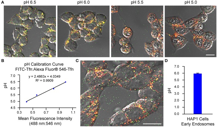
Figure 1
Use of confocal microscopy-based ratiometric measurement of fluorescent conjugates of transferrin to determine the pH of early endosomes in HAP1 cells. HAP1 cells were treated as described in the step...
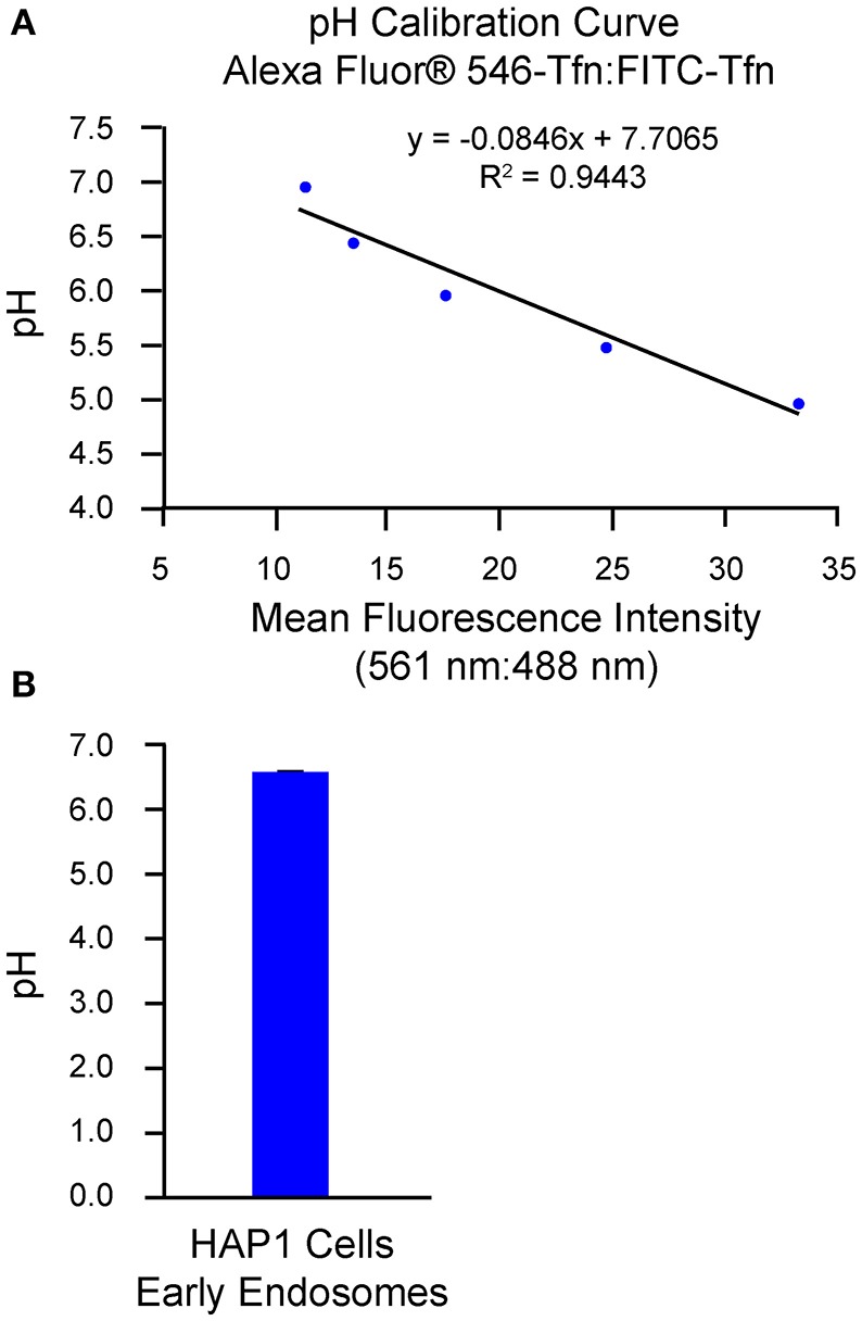
Figure 2
Use of flow cytometry-based/FACS-based ratiometric measurement of fluorescent conjugates of transferrin to determine the pH of early endosomes in HAP1 cells. HAP1 cells were treated as described in th...
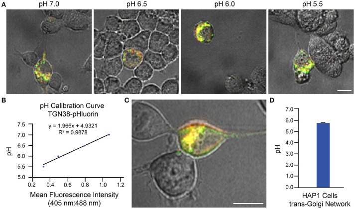
Figure 3
Determination of Golgi pH in HAP1 cells based on use of TGN38-pHluorin and ratiometric fluorescence microscopy. HAP1 cells were transfected with a plasmid encoding for TGN38-pHluorin and subsequently ...
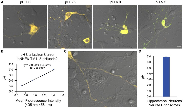
Figure 4
Determination of endosomal pH in neurites of mouse primary hippocampal neurons based on use of ratiometric pHluorin-tagged NHE6 and ratiometric fluorescence microscopy. Mouse primary hippocampal neuro...
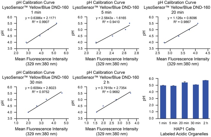
Figure 5
Measurement of intraorganellar pH in HAP1 cells using the ratiometric dye LysoSensoru2122 Yellow/Blue DND-160 and a microplate reader. HAP1 cells were treated as described in the stepwise procedures w...
Figure images are served from the NIH/NLM PubMed Central Open Access Subset or Europe PMC; copyright remains with the publishers and authors.
💬 Discussion
0 commentsNo comments yet. Be the first to start a discussion!
Leave a Comment