Abstract
AbstractA single subanesthetic dose of ketamine, an NMDA receptor antagonist, leads to fast-acting antidepressant effects. In rodent models, systemic ketamine is associated with higher dendritic spine density in the prefrontal cortex, reflecting structural remodeling that may underlie the behavioral changes. However, turnover of dendritic spines is a dynamic processin vivo, and the longitudinal effects of ketamine on structural plasticity remain unclear. The purpose of the current study is to use subcellular resolution optical imaging to determine the time course of dendritic alterationsin vivofollowing systemic ketamine administration in mice. We used two-photon microscopy to visualize repeatedly the same set of dendritic branches in the mouse medial frontal cortex (MFC) before and after a single injection of ketamine or saline. Compared to controls, ketamine-injected mice had higher dendritic spine density in MFC for up to 2 weeks. This prolonged increase in spine density was driven by an elevated spine formation rate, and not by changes in the spine elimination rate. A fraction of the new spines following ketamine injection was persistent, which is indicative of functional synapses. In a few cases, we also observed retraction of distal apical tuft branches on the day immediately after ketamine administration. These results indicate that following systemic ketamine administration, certain dendritic inputs in MFC are removed immediately, while others are added gradually. These dynamic structural modifications are consistent with a model of ketamine action in which the net effect is a rebalancing of synaptic inputs received by frontal cortical neurons.
🔬 Techniques
💻 Software
✨ Fluorophores
🧪 Sample Preparation
🏭 Microscope Brands
🧪 Reagent Suppliers
🔴 Lasers
💻 Software Details
🏷️ Research Resource Identifiers (RRIDs)
Verified research resources used in this paper:
🏛️ Research Organizations (ROR)
Affiliated research institutions:
📋 Methods
Mice
All animal procedures were performed in accordance with the regulations of the Yale University animal care committee. Experiments were performed on adult (postnatal day 73–149) Thy1-GFP-M ( n = 13; #007788, The Jackson Laboratory, RRID:IMSR_JAX:007788) and Thy1-YFP-H transgenic mice ( n = 3; #003782, The Jackson Laboratory, RRID:IMSR_JAX:003782). Mice of both sexes were used. Mice were housed under controlled temperature on a 12 h light/dark cycle with siblings (one to five per cage) and nesting material.
Surgery
Anesthesia was induced with a 2% isoflurane and oxygen mixture, which was lowered to 1.5% for the remainder of the surgery. Mice were secured by ear bars in a stereotaxic frame. Their body temperature was regulated with a hot water circulation pad. Mice were injected with carprofen (5 mg/kg, s.c.; catalog #024751, Butler Schein Animal Health) and dexamethasone (40 mg/kg, i.m.; catalog #D4902, Sigma-Aldrich) prior to surgery. A 2- to 3-mm-diameter craniotomy was made over the right medial frontal cortex (AP = 1.5 mm, ML = 0.5 mm) with a handheld dental drill. After the skull was carefully removed, the surface of the brain was irrigated with an artificial cerebrospinal fluid (ACSF; in m m : 5 KCl, 5 HEPES, 135 NaCl, 1 MgCl2, and 1.8 CaCl2, pH 7.3) until bleeding subsides. A drop of warmed, low-melting point agarose solution (2% in ACSF; Type III-A, High EEO agarose, catalog #A9793, Sigma-Aldrich) was applied over the craniotomy. A two-layer glass plug was fabricated by first etching out a 2-mm-diameter circle from a #0 thickness glass coverslip, then bonded with UV-activated epoxy (NT37-322, Edmund Optics) to a #1 thickness, 3-mm-diameter round glass coverslip (catalog #64-0720-CS-3R, Warner Instruments). The glass plug was placed over the craniotomy and held in place until the agarose solidifies. The glass plug was then stabilized by applying light pressure and adding superglue around the edges. A stainless steel head plate was affixed to the skull using C&B-METABOND (Parkell Inc.). Mice were given another dose of carprofen (5 mg/kg, s.c.) immediately after surgery and for each of the following 3 d (5 mg/kg, i.p.). Mice were given a period of at least 3 weeks to recover before imaging begins.
Show full methods section
Mice
All animal procedures were performed in accordance with the regulations of the Yale University animal care committee. Experiments were performed on adult (postnatal day 73–149) Thy1-GFP-M ( n = 13; #007788, The Jackson Laboratory, RRID:IMSR_JAX:007788) and Thy1-YFP-H transgenic mice ( n = 3; #003782, The Jackson Laboratory, RRID:IMSR_JAX:003782). Mice of both sexes were used. Mice were housed under controlled temperature on a 12 h light/dark cycle with siblings (one to five per cage) and nesting material.
Surgery
Anesthesia was induced with a 2% isoflurane and oxygen mixture, which was lowered to 1.5% for the remainder of the surgery. Mice were secured by ear bars in a stereotaxic frame. Their body temperature was regulated with a hot water circulation pad. Mice were injected with carprofen (5 mg/kg, s.c.; catalog #024751, Butler Schein Animal Health) and dexamethasone (40 mg/kg, i.m.; catalog #D4902, Sigma-Aldrich) prior to surgery. A 2- to 3-mm-diameter craniotomy was made over the right medial frontal cortex (AP = 1.5 mm, ML = 0.5 mm) with a handheld dental drill. After the skull was carefully removed, the surface of the brain was irrigated with an artificial cerebrospinal fluid (ACSF; in m m : 5 KCl, 5 HEPES, 135 NaCl, 1 MgCl2, and 1.8 CaCl2, pH 7.3) until bleeding subsides. A drop of warmed, low-melting point agarose solution (2% in ACSF; Type III-A, High EEO agarose, catalog #A9793, Sigma-Aldrich) was applied over the craniotomy. A two-layer glass plug was fabricated by first etching out a 2-mm-diameter circle from a #0 thickness glass coverslip, then bonded with UV-activated epoxy (NT37-322, Edmund Optics) to a #1 thickness, 3-mm-diameter round glass coverslip (catalog #64-0720-CS-3R, Warner Instruments). The glass plug was placed over the craniotomy and held in place until the agarose solidifies. The glass plug was then stabilized by applying light pressure and adding superglue around the edges. A stainless steel head plate was affixed to the skull using C&B-METABOND (Parkell Inc.). Mice were given another dose of carprofen (5 mg/kg, s.c.) immediately after surgery and for each of the following 3 d (5 mg/kg, i.p.). Mice were given a period of at least 3 weeks to recover before imaging begins.
Imaging
Mice were anesthetized with 1.5% isoflurane and head fixed. Temperature was regulated using a heating pad with rectal probe feedback. The two-photon microscope (Movable Objective Microscope, Sutter Instrument) was controlled using the ScanImage software ( Pologruto et al., 2003 , RRID:SCR_014307). Excitation was provided by an ultrafast laser (Chameleon Ultra II, Coherent) and focused with a high-numerical aperture microscope objective (XLUMPLFLN20X/1.0, Olympus). For imaging green fluorescent protein (GFP)- or yellow fluorescent protein (YFP)-expressing dendrites, excitation wavelength was set at 920 nm, and emission was collected behind a bandpass filter from 475 to 550 nm. Each mouse was injected with either ketamine (10 mg/kg, i.p.) or saline vehicle on a non-imaging day. To investigate short-term effects, mice were imaged on days −3, −1, and 1 relative to the day of injection. For long-term studies, mice were imaged on days −3, −1, 1, 3, 5, 10, and 15 relative to the day of injection. Multiple fields of view were imaged in the same mouse. The same field of view was identified across days by finding landmark structures such as blood vessels or an edge of the glass window. At each field of view, image stacks were acquired at 1024 × 1024 pixels, spanning a field of view of 60.5 × 60.5 μm, and at 2 μm steps for a z -range of 20–30 μm. Each imaging session lasted up to 2.5 h. Although we did not explicitly record the duration of imaging sessions, we estimated post hoc based on the acquisition times of the first and last image files in the computer.
Image analysis
In all of the figures, we are presenting the raw images with only adjustments to the black-and-white levels (linear), with no modification to contrast (nonlinear) or removal of neighboring axons, or any other manipulations. Initially, image stacks were processed for motion correction using the StackReg plug-in ( Thévenaz et al., 1998 , RRID:SCR_014308) in ImageJ ( Schneider et al., 2012 , RRID:SCR_003070). Then, structural parameters were analyzed from each image stack using ImageJ. The physical parameters of dendritic spines were characterized based on criteria established in a standardized protocol ( Holtmaat et al., 2009 ). Briefly, dendritic spines were counted if the protrusions extended at least 0.4 μm away from the shaft. Dendritic spine length was the distance from the base at the shaft to the tip. Dendritic spine head diameter was the width at the widest extent of the spine. Distances were measured using the line segment tool in ImageJ. The dendritic spine formation rate was defined as the number of new spine protrusions observed in two consecutive imaging sessions divided by the total number of dendritic spines in the first imaging session. To assess longitudinal changes in the spine formation rate, we calculated the difference from baseline by subtracting the formation rate of each field of view by the baseline rate of the subject. The baseline rate of each subject was estimated by averaging the spine formation rates of all fields of view imaged from the same individual prior to injection (i.e. between days −3 and −1). The dendritic elimination rate was quantified using the same procedure for spine protrusions that disappeared. Most of the sessions were imaged 2 d apart, but some sessions were imaged 5 d apart (i.e., days 5–10 and days 10–15). Presumably, with the same spine formation rate, we would observe more new spines in sessions occurring 5 d apart relative to those occurring 2 d apart because more time has elapsed. Therefore, when estimating the spine formation/elimination rate from new/lost spine counts, we report turnover rates for sessions occurring 5 d apart with a correction factor, by multiplying the measured rates by two-fifths. For the apical tuft branches, dendritic segments were traced over using the freehand line tool, and then summed for total length in ImageJ. To assess longitudinal changes of the imaged dendritic segments, we calculated the fold change from the last session for each field of view by dividing the measured branch length of an imaging session by that of the prior imaging session.
Statistics
We performed statistical tests considering fields of view as independent samples. This is a major assumption, justified in part by the fact that the fields of view were at random, nonoverlapping locations and that each one comprises a very small portion (0.06%) of the window area of each mouse. The reason for making this assumption is that a different number of fields of view was obtained for each mouse, so if we compare subjects only, the results will have a bias for those with fewer fields of view. To ensure that this assumption does not affect the major conclusions of the study, we repeated statistical tests in data from three sessions considering each mouse as a sample when possible. For all longitudinal results, two-way mixed ANOVA with repeated measures was used to test the factors contributing to changes in spine density, dendritic branch length, spine formation rate, and spine elimination rate. The factors were treatment (with ketamine or saline; between-subject), day (within-subject), and their interaction. The two-tailed t test was used to compare means that did not involve multiple days. The two-sample Kolmogorov–Smirnov test was used to compare cumulative distributions. Data are reported as the mean ± SEM. Table 1 contains a list of the statistical tests performed, p values, and sample sizes. p values and sample sizes are reported instead of observed power to provide more information on the samples involved and because the p values are directly related to the observed power. Table 1: Statistical table Data structure Test Exact p value N a Spine density Two-factor, btw (treatment) and win (day) rANOVA Treatment: p = 6 × 10 −7 ; day: p = 0.40; interaction: p = 0.39 28/25 fields of view for 7 sessions for ket vs saline b Spine formation rate Two-factor, btw (treatment) and win (day) rANOVA Treatment: p = 0.03; day: p = 0.001; interaction: p = 0.03 58/97 fields of view for 3 sessions for ket vs saline c Spine elimination rate Two-factor, btw (treatment) and win (day) rANOVA Treatment: p = 0.9; day: p = 0.003; interaction: p = 0.9 58/97 fields of view for 3 sessions for ket vs saline d Spine formation rate Two-factor, btw (treatment) and win (day) rANOVA Treatment: p = 2 × 10 −4 ; day: p = 0.5; interaction: p = 0.08 28/25 fields of view for 7 sessions for ket vs saline e Spine elimination rate Two-factor, btw (treatment) and win (day) rANOVA Treatment: p = 0.1; day: p = 0.001; interaction: p = 0.07 28/25 fields of view for 7 sessions for ket vs saline f Field of view fraction Normally distributed χ 2 test p = 0.005 58/97 fields of view for ket vs saline g Spine density Two-factor, btw (treatment) and win (day) rANOVA Treatment: p = 0.007; day: p = 0.87; interaction: p = 0.98 8/8 mice for ket vs saline h Spine formation rate Two-factor, btw (treatment) and win (day) rANOVA Treatment: p = 0.07; day: p = 0.20; interaction: p = 0.69 8/8 mice for ket vs saline i Spine elimination rate Two-factor, btw (treatment) and win (day) rANOVA Treatment: p = 0.64; day: p = 0.23; interaction: p = 0.62 8/8 mice for ket vs saline j Persistent fraction Normally distributed Two-tailed t test p = 0.3 28/25 fields of view for ket vs saline k Persistent fraction Normally distributed Two-tailed paired t test p = 0.007 28 fields of view for ket m Persistent fraction Normally distributed Two-tailed paired t test p = 0.002 28 fields of view for ket n Persistent fraction Normally distributed Two-tailed paired t test p = 0.1 25 fields of view for saline o Persistent fraction Normally distributed Two-tailed paired t test p = 0.9 25 fields of view for saline p Spine head length Normally distributed Two-tailed paired t test p = 0.02 328/328 new vs existing spines q Spine head width Normally distributed Two-tailed paired t test p = 3 × 10 −5 328/328 new vs existing spines r Spine head length Cumulative fractions Two-sample Kolmogorov–Smirnov test p = 9 × 10 −6 328/328 new vs existing spines s Spine head width Cumulative fractions Two-sample Kolmogorov–Smirnov test p = 4 × 10 −4 328/328 new vs existing spines t Spine head length Cumulative fractions Two-sample Kolmogorov–Smirnov test p = 0.9 61/328 spines for pre-ket vs post-ket u Spine head length Cumulative fractions Two-sample Kolmogorov–Smirnov test p = 0.09 61/328 spines for pre-ket vs post-ket v Spine head width Cumulative fractions Two-sample Kolmogorov–Smirnov test p = 0.2 61/328 spines for pre-ket vs post-ket w Spine head width Cumulative fractions Two-sample Kolmogorov–Smirnov test p = 0.5 61/328 spines for pre-ket vs post-ket x Dendrite length Two-factor, btw (treatment) and win (day) rANOVA Treatment: p = 1 × 10 −12 ; day: p = 0.02; interaction: p = 0.02 28/25 fields of view for 7 sessions for ket vs saline y Dendrite length and formation rate Two variables: binary (with or without branch loss) and continuous (formation rate) Regression coefficient p = 0.2 28 fields of view for ket z Dendrite length and elimination rate Two variables: binary (with or without branch loss) and continuous (elimination rate) Regression coefficient p = 0.3 28 fields of view for ket aa Branch width of imaged dendritic segments Normally distributed Two-tailed t test p = 0.44 117 stable and 16 retracted dendritic segments ab Dendrite length Two-factor, btw (treatment) and win (day) rANOVA Treatment: p = 0.003; day: p = 0.69; interaction: p = 0.69 8/8 mice for ket vs saline ac Change in dendritic spine density Non-parametric Wilcoxon ranked-sum p = 1 8/8 mice for ket vs saline ad Change in dendritic spine density Non-parametric Wilcoxon ranked-sum p = 0.3 5 female and 11 male mice ae Change in dendritic spine density Two continuous variables Regression coefficient p = 0.8 16 mice af Change in dendritic spine density Two continuous variables Regression coefficient p = 0.8 16 mice ag Change in dendritic spine density Two continuous variables Regression coefficient p = 0.16 16 mice rANOVA, repeated measures ANOVA; btw, between-factor of the ANOVA; win, within-factor of the ANOVA; ket, ketamine administration; saline, saline administration.
📊 Figures
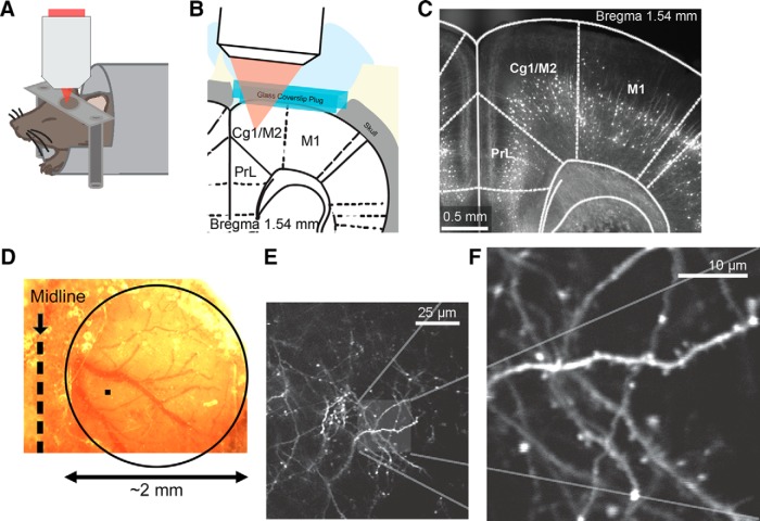
Figure 1.
Longitudinal imaging of dendritic architecture in the mouse medial frontal cortex. A , Schematic of the imaging experiment. B , Schematic of the long-term window implant. C , Fluorescence image of a f...
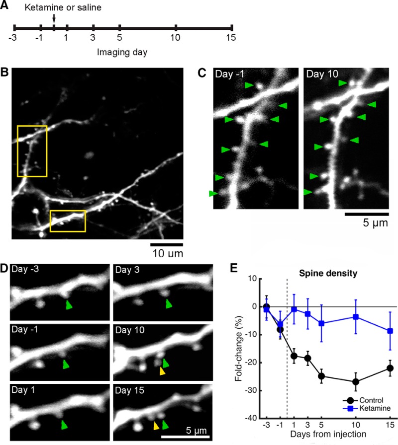
Figure 2.
Systemic ketamine administration leads to higher dendritic spine density for at least 2 weeks relative to that of controls. A , Time line of the experiment. Ketamine was administered at a dose of 10 m...
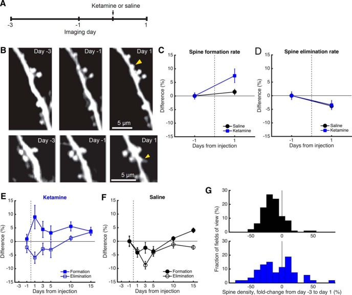
Figure 3.
Higher spine density is due to an elevated rate of spine formation. A , Time line of the experiment. Ketamine was administered at a dose of 10 mg/kg through intraperitoneal injection. B , Images of tw...
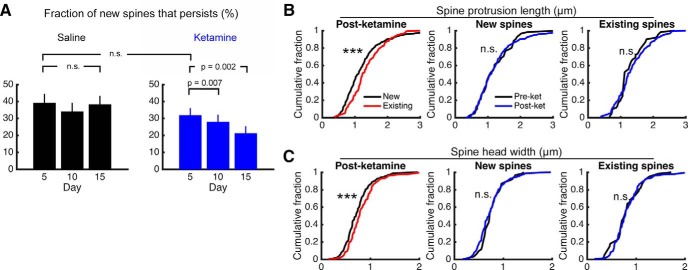
Figure 4.
Newly formed protrusions following systemic ketamine administration are consistent with nascent spines. A , The fraction of newly formed spines found on day 1 that could be observed again on day 5, 10...
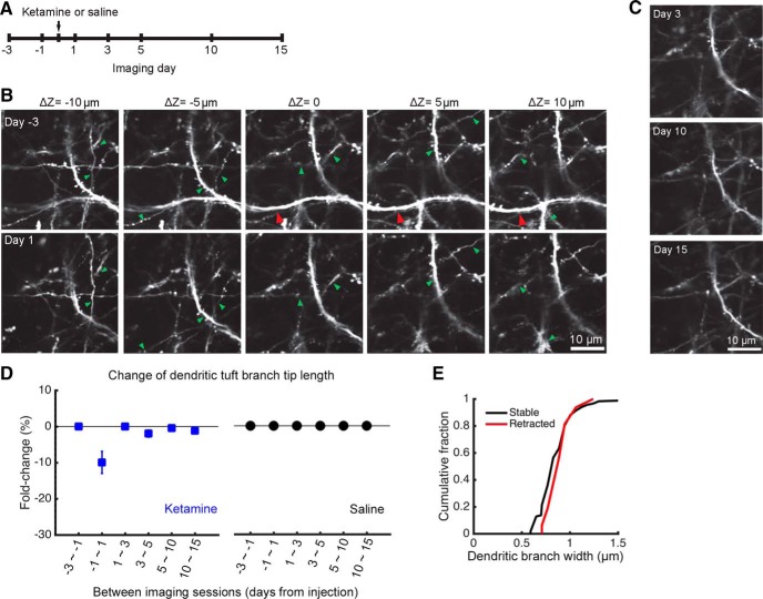
Figure 5.
Systemic ketamine administration associated with the retraction of distal apical tuft branches. A , Time line of the experiment. Ketamine was administered at a dose of 10 mg/kg through intraperitoneal...
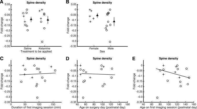
Figure 6.
Potential factors contributing to the decline of dendritic spine density prior to injection. A , Fold change in dendritic spine density from day u22123 to day u22121 (preinjection) for mice to be inje...
Figure images are served from the NIH/NLM PubMed Central Open Access Subset or Europe PMC; copyright remains with the publishers and authors.
💬 Discussion
0 commentsNo comments yet. Be the first to start a discussion!
Leave a Comment