Abstract
This paper reviews some of the challenges posed by the huge growth of experimental data generated by the new generation of large-scale experiments at UK national facilities at the Rutherford Appleton Laboratory (RAL) site at Harwell near Oxford. Such ‘Big Scientific Data’ comes from the Diamond Light Source and Electron Microscopy Facilities, the ISIS Neutron and Muon Facility and the UK's Central Laser Facility. Increasingly, scientists are now required to use advanced machine learning and other AI technologies both to automate parts of the data pipeline and to help find new scientific discoveries in the analysis of their data. For commercially important applications, such as object recognition, natural language processing and automatic translation, deep learning has made dramatic breakthroughs. Google's DeepMind has now used the deep learning technology to develop their AlphaFold tool to make predictions for protein folding. Remarkably, it has been able to achieve some spectacular results for this specific scientific problem. Can deep learning be similarly transformative for other scientific problems? After a brief review of some initial applications of machine learning at the RAL, we focus on challenges and opportunities for AI in advancing materials science. Finally, we discuss the importance of developing some realistic machine learning benchmarks using Big Scientific Data coming from several different scientific domains. We conclude with some initial examples of our ‘scientific machine learning’ benchmark suite and of the research challenges these benchmarks will enable. This article is part of a discussion meeting issue ‘Numerical algorithms for high-performance computational science’.
🔬 Techniques
💻 Software Details
🏛️ Research Organizations (ROR)
Affiliated research institutions:
📋 Methods
3. Machine learning and materials science (a) Overview of materials science and machine learning Machine learning has started to change the way that we do materials science, contributing to accelerated characterization, synthesis and modelling. These advances are driven by the availability of easy-to-use packages for building machine learning models, e.g. Scikit-Learn [ 32 ] and Keras [ 33 ], as well as a recent proliferation of publicly available datasets, resulting in a materials science ‘ImageNet moment’ where the availability of data fuels a step-change in data-driven approaches. We will briefly survey some of the cutting-edge machine learning works in the areas of materials discovery and characterization and outline some of the work of the SciML team that is using machine learning to analyse the data produced at the UK's large national scientific facilities. Computational materials science dates back to mid-twentieth century, an early example being the quantum chemistry exchange programme, which allowed experimental chemists to perform quantum chemical calculations with relative ease [ 34 ]. At this early stage, the paradigm of computational materials science was to use computational methods to help interpret experimental results by doing a few expensive calculations on materials whose structure was already well known.
Density functional theory
(DFT) was popularized by Walter Kohn and co-workers in the 1960s; with the advent of powerful super-computers in the late-twentieth century performing several DFT calculations suddenly became feasible [ 35 , 36 ]. Structure prediction methods based on global optimization algorithms, such as particle swarm optimization and genetic algorithms, mean that it is now possible to predict the structure and properties for new materials starting from the composition alone [ 37 ]. The availability of rapid and accurate DFT calculations has facilitated the development of large, high-quality databases of calculated materials properties, for example the Materials Project, Aflow, Open Quantum Materials Database and Nomad [ 38 ]. The sudden availability of these datasets is revolutionizing the way that data-driven approaches are used in materials science. Figure 4 plots the number of publications containing ‘machine learning materials' from the Web of Science. We indicate on the figure dates that some notable databases became available, suggestive of the important role of these datasets in driving the development of a new paradigm of computational materials science [ 39 ]. Figure 4. The ML explosion in materials science. The number of papers containing the terms machine learning and materials are plotted on a bar chart. We indicate the dates of materials data repositories becoming available and plot the number of citations for popular machine learning toolkit, Scikit-Learn over the same period. (Online version in colour.) New machine learning approaches trained on computational databases are capable of making rapid and accurate predictions of materials properties by considering composition alone. The electronic band gap is a good example of a material property that is important in a range of applications from microelectronics to photovoltaics. Several studies have reported machine learning algorithms that are capable of predicting the band gap of a material from its composition [ 40 – 42 ]. These kinds of algorithms can be incorporated into materials discovery workflows and have recently been applied to the prediction of new photoactive Earth-abundant materials for photocatalysis [ 43 ]. Generative models, using neural networks, are also now being used to postulate new molecular materials [ 44 ]. For example, the long short-term memory (LSTM) neural network architecture has recently been shown to be able to predict new drug molecules using greatly reduced training data compared to other approaches [ 45 ]. In the ORGAN project, a combination of generative adversarial network and reinforcement learning combine to bias molecular generation algorithms towards desired final metrics, potentially allowing the automated design of a molecule to meet a specific property [ 46 ]. Interpretation of complicated experimental spectra has regularly relied on the calculations for clarification, but now with databases of calculated properties available it is possible to develop machine learning algorithms to interpret spectra in an automated way, free from human bias and capable of identifying signals which are missed during manual inspection. A powerful recent example is in the field of X-ray absorption spectroscopy (XAS) where a dataset of calculated spectra was recently made available [ 47 ]. Calculated spectra have been used to train neural networks, which are facilitating an unprecedented analysis of materials datasets, for example, in characterizing structural transformations in materials, in making on-the-fly predictions about the presence of chemical environments in a sample and in identifying sub-nanometer atomic assemblies [ 48 – 50 ]. Recently, an ensemble learning algorithm trained on this dataset, that is capable of identifying the oxidation state and coordination environment in a diverse range of chemistries, has been made publicly available [ 51 ]. (b) Machine learning and experimental materials data The rapidly expanding capability of large-scale facilities to analyse material samples means that the demand for robust, automated, on-the-fly analysis is becoming ever more pressing. Examples, such as the XAS studies described above, show how a fusion of experiment, simulated data and machine learning algorithms can facilitate the rapid interpretation of these rich new data sources. In the SciML team, we are developing a range of machine learning algorithms for materials data analysis. Inspired and challenged by the progress in machine learning at other large-scale facilities outlined in the start of §2, we have started to build a machine learning capability at the RAL for the analysis of materials science data collected on site. Here, we present our work on diffuse multiple scattering (DMS) experiments at the Diamond Light Source and on inelastic neutron scattering experiments at ISIS neutron and muon source. (i) Diffuse multiple scattering DMS is a relatively new crystallographic technique and has been made possible by the immense increase in the flux of modern synchrotron sources and modern detector systems [ 52 ]. DMS can be a powerful technique for allowing measurement of fine details such as lattice strain and for following structural phase transitions in materials. However, the detailed experimental set-up requires expert knowledge and several time-consuming steps, which limit the routine application of the technique. One of the parameters that must be known for the experimental analysis of DMS data is the azimuthal angle of the sample, which is not known a priori and determines the values at which reciprocal crystal lattice vectors cross the Ewald sphere, as defined in [ 52 ]. We have trained a neural network consisting of convolutional and densely connected layers to predict the azimuthal angle of the sample based on the observed scattering pattern. Typically, determination of the azimuthal angle is a time-consuming task, requiring expert knowledge and representing a serious bottleneck for the application of DMS. We have built a database of 250 000+ simulated patterns, Ψ (R) T, using the DMS Python code, which are used to train the neural network [ 52 ]. The simulated patterns provide a labelled ground truth of azimuthal angles, as a function of the patterns Ψ (R) T . We then train our NN to predict Ψ based on the input image R , updating the filters, weights and biases of the NN to minimize the difference between predicted Ψ (R) NN and Ψ (R) T . The NN that we train is then capable of predicting the azimuthal angle to be within 6.5° ( figure 5 ). The NN, once trained, can provide an answer in a fraction of the time required for exhaustive comparison of images. Figure 5. A schematic of the CNN used to predict coupling azimuthal angle from DMS images. A two-dimensional map of multiple scattering lines is passed through two convolutional layers, flattened and passed through two densely connected layers and finally passed to a single-output node for Ψ . Note that the numbers of filters and nodes are just for illustration, see methods section on DMS network for details. (Online version in colour.) DMS network methods: The NN used for predicting the azimuthal angle of a DMS sample consists of convolutional and densely connected layers. The first convolutional layer contains 32 3 × 3 kernel filters, followed by a maxpooling of 2 × 2; the second convolutional layer contains 64 3 × 3 filters, followed by maxpooling of 2 × 2. We include a dropout rate of 0.2 between the convolutional layers to guard against over-fitting. The two-dimensional data are then flattened and fed into a densely connected layer of 32 nodes, connected to a densely connected layer of 16 nodes. The final hidden layer is connected to a single-output node with a linear activation function to allow the network to perform regression. All hidden layers are connected with rectified linear unit (ReLU) activation functions. The network is trained on 75% of the dataset and then validated on the remaining 25%. The training and validation curves are shown in figure 6 . Figure 6. Training and validation scores for the mean absolute error for the prediction of the azimuthal angle of a DMS pattern. (Online version in colour.) (ii) Magnon neutron scattering Inelastic neutron scattering can provide detailed information about microscopic materials structure. In particular, the magnetic moment of neutrons allows one to probe the magnetic structure and ordering in a material. In this example, we have investigated the use of NNs for predicting the magnetic coupling constants ( J ) in Rb 2 MnF 4 . Rb 2 MnF 4 is a near-ideal two-dimensional, spin 5/2 Heisenberg antiferromagnet and has been used extensively to test predictions for the two-dimensional Heisenberg quantum Hamiltonian [ 53 , 54 ]. As such, this system provides an ideal test case for exploring the ability of an NN for this task. Rb 2 MnF 4 consists of planes of MnF 2 layers, with magnetic Mn arranged in a square lattice. Experimentally, it has been established that Rb 2 MnF 4 has a magnetic coupling between nearest neighbour Mn sites with a coupling constant variously measured as J = 0.648 ± 0.003, 0.6544 ± 0.014 and 0.673 ± 0.028 meV depending on the experiment and fitting model [ 53 , 54 ]. A careful examination of the spin wave energies along the antiferromagnetic zone boundary reveals that in addition to the nearest neighbour coupling, there is a next-nearest neighbour term in the Hamiltonian J′, which has been measured to be 0.006 ± 0.003 and 0.012 ± 0.002 meV in different experiments [ 54 , 55 ]. In our study, we built a training set of 29 957 simulated spin wave spectra in the two-dimensional ( h , k , 0) plane from 0 ≤ h , k < 1 of Rb 2 MnF 4 using the SpinW code [ 56 ]. This serves as our labelled training set R . We then train our NN to learn the relation between R and ( J , J ′ ) ; ( J , J ′) = f ( R ), where the function f is the NN. After training (details below), we obtain a NN that has a mean average error of ±0.0055 meV on J and±0.0036 meV on J ′, using data that was not included in the training set. As a true test of the NN, we provided experimental data collected on the MARI instrument at the ISIS neutron and muon source. The data were collected on a sample of Rb 2 MnF 4 and the image of the integrated energy over the plane is shown in figure 7 . Figure 7. A schematic of the CNN used to predict coupling constants from inelastic neutron scattering images. A two-dimensional map of integrated energy is passed through four convolutional layers, flattened and densely connected to two output nodes for J and J ′. Note numbers of filters and nodes are just for illustration, see methods section on Magnon network for details. (Online version in colour.) The NN trained on simulated data predicts a value of J = 0.6763 meV and J ′ = 0.0104 meV for the experimental spectrum, in excellent agreement with previous experimental results. This demonstrates the ability of a convolutional NN to learn to predict magnetic coupling constants from simulated data, even picking up subtle, difficult-to-spot features, such as the value of the next-nearest-neighbour coupling constant J ′. We stress here that prior knowledge was used to select a training set representative of a reasonable range of final values together with our intuition about the number of coupling constants present. This fusion of prior knowledge and NN architectures helps to improve the efficiency of training greatly and allows the development of high-quality models with significantly less data than would be otherwise required. We consider this an example of how NN can be used to augment existing expertise and assist in difficult analysis where some prior knowledge already exists. Magnon network methods: The NN used for predicting the magnetic coupling constants consists of four convolutional layers terminated by a densely connected layer. The first convolutional layer contains 32 3 × 3 kernel filters; the second convolutional layer contains 64 3 × 3 filters; the third convolutional layer contains 32 3 × 3 kernel filters; and the final convolutional layer contains 16 3 × 3 kernel filters. All convolutional layers are followed by maxpooling of 2 × 2. The two-dimensional data are then flattened and fed into a densely connected layer of two nodes with a linear activation function to allow the network to perform regression. All hidden layers are connected with ReLU activation functions. The network is trained on 27 000 images of the dataset and then validated on the remaining 2957 images. The training and validation curves are shown in figure 8 . Before feeding the simulated images into the network, they are converted to a two-dimensional histogram of 128 × 128, and we apply a mask to the simulated data to cover the regions of the pattern that are not recorded due to the detector geometry—these appear as areas of purple in the image in figure 7 . Figure 8. Training and validation scores for the mean absolute error for the prediction of the coupling constants from an inelastic neutron scattering pattern. (Online version in colour.) (c) Further work In the examples given here, we have used convolutional neural networks (CNNs) to analyse spectra and patterns collected at synchrotron facilities and represented as images. Deep CNNs have revolutionized the field of image processing and recognition in many fields of business and research. As alluded to earlier, the explosion in the popularity of NNs, and in particular of deep CNNs for image applications, has been driven largely by the availability of large labelled datasets for training. Deep CNNs typically rely on the combinations of many types of operation and connection to achieve their most powerful results on the most difficult problems. This results in networks that not only require vast amounts of labelled data but also have many tuneable hyper-parameters. This can hamper the application in many materials science problems, where labelled datasets are limited. Recently, a new type of image recognition architecture, the mixed-scale dense MSD-NN neural network, was introduced by researchers at Berkeley Laboratory [ 57 ]. This architecture has several differences from traditional CNNs. The MSD-NN uses dilation filters rather than traditional convolutional kernels, which means that longer range correlations in images can be captured, depending on dilation settings ( figure 9 ). In the MSD-NN, all convolved layers are fully connected, unlike a CNN where layers connect sequentially. This full connectivity means that the network does not have to remember information from layer to layer for the final outcome. In the initial work, it has been shown that the MSD-NN can learn on significantly smaller datasets and with less hyper-parameter tuning than CNNs. In SciML, we are currently exploring the application of MSD-NNs for soft X-ray image segmentation and for a range of materials science classification problems. Figure 9. Top: an illustration of a typical convolution filter (left) which convolves information from neighbour pixels and a dilation filter (right) which can convolve with pixels further removed. Lower: a schematic of the fully connected mixed-dense neural network architecture. (Online version in colour.)
Show full methods section
3. Machine learning and materials science (a) Overview of materials science and machine learning Machine learning has started to change the way that we do materials science, contributing to accelerated characterization, synthesis and modelling. These advances are driven by the availability of easy-to-use packages for building machine learning models, e.g. Scikit-Learn [ 32 ] and Keras [ 33 ], as well as a recent proliferation of publicly available datasets, resulting in a materials science ‘ImageNet moment’ where the availability of data fuels a step-change in data-driven approaches. We will briefly survey some of the cutting-edge machine learning works in the areas of materials discovery and characterization and outline some of the work of the SciML team that is using machine learning to analyse the data produced at the UK's large national scientific facilities. Computational materials science dates back to mid-twentieth century, an early example being the quantum chemistry exchange programme, which allowed experimental chemists to perform quantum chemical calculations with relative ease [ 34 ]. At this early stage, the paradigm of computational materials science was to use computational methods to help interpret experimental results by doing a few expensive calculations on materials whose structure was already well known.
Density functional theory
(DFT) was popularized by Walter Kohn and co-workers in the 1960s; with the advent of powerful super-computers in the late-twentieth century performing several DFT calculations suddenly became feasible [ 35 , 36 ]. Structure prediction methods based on global optimization algorithms, such as particle swarm optimization and genetic algorithms, mean that it is now possible to predict the structure and properties for new materials starting from the composition alone [ 37 ]. The availability of rapid and accurate DFT calculations has facilitated the development of large, high-quality databases of calculated materials properties, for example the Materials Project, Aflow, Open Quantum Materials Database and Nomad [ 38 ]. The sudden availability of these datasets is revolutionizing the way that data-driven approaches are used in materials science. Figure 4 plots the number of publications containing ‘machine learning materials' from the Web of Science. We indicate on the figure dates that some notable databases became available, suggestive of the important role of these datasets in driving the development of a new paradigm of computational materials science [ 39 ]. Figure 4. The ML explosion in materials science. The number of papers containing the terms machine learning and materials are plotted on a bar chart. We indicate the dates of materials data repositories becoming available and plot the number of citations for popular machine learning toolkit, Scikit-Learn over the same period. (Online version in colour.) New machine learning approaches trained on computational databases are capable of making rapid and accurate predictions of materials properties by considering composition alone. The electronic band gap is a good example of a material property that is important in a range of applications from microelectronics to photovoltaics. Several studies have reported machine learning algorithms that are capable of predicting the band gap of a material from its composition [ 40 – 42 ]. These kinds of algorithms can be incorporated into materials discovery workflows and have recently been applied to the prediction of new photoactive Earth-abundant materials for photocatalysis [ 43 ]. Generative models, using neural networks, are also now being used to postulate new molecular materials [ 44 ]. For example, the long short-term memory (LSTM) neural network architecture has recently been shown to be able to predict new drug molecules using greatly reduced training data compared to other approaches [ 45 ]. In the ORGAN project, a combination of generative adversarial network and reinforcement learning combine to bias molecular generation algorithms towards desired final metrics, potentially allowing the automated design of a molecule to meet a specific property [ 46 ]. Interpretation of complicated experimental spectra has regularly relied on the calculations for clarification, but now with databases of calculated properties available it is possible to develop machine learning algorithms to interpret spectra in an automated way, free from human bias and capable of identifying signals which are missed during manual inspection. A powerful recent example is in the field of X-ray absorption spectroscopy (XAS) where a dataset of calculated spectra was recently made available [ 47 ]. Calculated spectra have been used to train neural networks, which are facilitating an unprecedented analysis of materials datasets, for example, in characterizing structural transformations in materials, in making on-the-fly predictions about the presence of chemical environments in a sample and in identifying sub-nanometer atomic assemblies [ 48 – 50 ]. Recently, an ensemble learning algorithm trained on this dataset, that is capable of identifying the oxidation state and coordination environment in a diverse range of chemistries, has been made publicly available [ 51 ]. (b) Machine learning and experimental materials data The rapidly expanding capability of large-scale facilities to analyse material samples means that the demand for robust, automated, on-the-fly analysis is becoming ever more pressing. Examples, such as the XAS studies described above, show how a fusion of experiment, simulated data and machine learning algorithms can facilitate the rapid interpretation of these rich new data sources. In the SciML team, we are developing a range of machine learning algorithms for materials data analysis. Inspired and challenged by the progress in machine learning at other large-scale facilities outlined in the start of §2, we have started to build a machine learning capability at the RAL for the analysis of materials science data collected on site. Here, we present our work on diffuse multiple scattering (DMS) experiments at the Diamond Light Source and on inelastic neutron scattering experiments at ISIS neutron and muon source. (i) Diffuse multiple scattering DMS is a relatively new crystallographic technique and has been made possible by the immense increase in the flux of modern synchrotron sources and modern detector systems [ 52 ]. DMS can be a powerful technique for allowing measurement of fine details such as lattice strain and for following structural phase transitions in materials. However, the detailed experimental set-up requires expert knowledge and several time-consuming steps, which limit the routine application of the technique. One of the parameters that must be known for the experimental analysis of DMS data is the azimuthal angle of the sample, which is not known a priori and determines the values at which reciprocal crystal lattice vectors cross the Ewald sphere, as defined in [ 52 ]. We have trained a neural network consisting of convolutional and densely connected layers to predict the azimuthal angle of the sample based on the observed scattering pattern. Typically, determination of the azimuthal angle is a time-consuming task, requiring expert knowledge and representing a serious bottleneck for the application of DMS. We have built a database of 250 000+ simulated patterns, Ψ (R) T, using the DMS Python code, which are used to train the neural network [ 52 ]. The simulated patterns provide a labelled ground truth of azimuthal angles, as a function of the patterns Ψ (R) T . We then train our NN to predict Ψ based on the input image R , updating the filters, weights and biases of the NN to minimize the difference between predicted Ψ (R) NN and Ψ (R) T . The NN that we train is then capable of predicting the azimuthal angle to be within 6.5° ( figure 5 ). The NN, once trained, can provide an answer in a fraction of the time required for exhaustive comparison of images. Figure 5. A schematic of the CNN used to predict coupling azimuthal angle from DMS images. A two-dimensional map of multiple scattering lines is passed through two convolutional layers, flattened and passed through two densely connected layers and finally passed to a single-output node for Ψ . Note that the numbers of filters and nodes are just for illustration, see methods section on DMS network for details. (Online version in colour.) DMS network methods: The NN used for predicting the azimuthal angle of a DMS sample consists of convolutional and densely connected layers. The first convolutional layer contains 32 3 × 3 kernel filters, followed by a maxpooling of 2 × 2; the second convolutional layer contains 64 3 × 3 filters, followed by maxpooling of 2 × 2. We include a dropout rate of 0.2 between the convolutional layers to guard against over-fitting. The two-dimensional data are then flattened and fed into a densely connected layer of 32 nodes, connected to a densely connected layer of 16 nodes. The final hidden layer is connected to a single-output node with a linear activation function to allow the network to perform regression. All hidden layers are connected with rectified linear unit (ReLU) activation functions. The network is trained on 75% of the dataset and then validated on the remaining 25%. The training and validation curves are shown in figure 6 . Figure 6. Training and validation scores for the mean absolute error for the prediction of the azimuthal angle of a DMS pattern. (Online version in colour.) (ii) Magnon neutron scattering Inelastic neutron scattering can provide detailed information about microscopic materials structure. In particular, the magnetic moment of neutrons allows one to probe the magnetic structure and ordering in a material. In this example, we have investigated the use of NNs for predicting the magnetic coupling constants ( J ) in Rb 2 MnF 4 . Rb 2 MnF 4 is a near-ideal two-dimensional, spin 5/2 Heisenberg antiferromagnet and has been used extensively to test predictions for the two-dimensional Heisenberg quantum Hamiltonian [ 53 , 54 ]. As such, this system provides an ideal test case for exploring the ability of an NN for this task. Rb 2 MnF 4 consists of planes of MnF 2 layers, with magnetic Mn arranged in a square lattice. Experimentally, it has been established that Rb 2 MnF 4 has a magnetic coupling between nearest neighbour Mn sites with a coupling constant variously measured as J = 0.648 ± 0.003, 0.6544 ± 0.014 and 0.673 ± 0.028 meV depending on the experiment and fitting model [ 53 , 54 ]. A careful examination of the spin wave energies along the antiferromagnetic zone boundary reveals that in addition to the nearest neighbour coupling, there is a next-nearest neighbour term in the Hamiltonian J′, which has been measured to be 0.006 ± 0.003 and 0.012 ± 0.002 meV in different experiments [ 54 , 55 ]. In our study, we built a training set of 29 957 simulated spin wave spectra in the two-dimensional ( h , k , 0) plane from 0 ≤ h , k < 1 of Rb 2 MnF 4 using the SpinW code [ 56 ]. This serves as our labelled training set R . We then train our NN to learn the relation between R and ( J , J ′ ) ; ( J , J ′) = f ( R ), where the function f is the NN. After training (details below), we obtain a NN that has a mean average error of ±0.0055 meV on J and±0.0036 meV on J ′, using data that was not included in the training set. As a true test of the NN, we provided experimental data collected on the MARI instrument at the ISIS neutron and muon source. The data were collected on a sample of Rb 2 MnF 4 and the image of the integrated energy over the plane is shown in figure 7 . Figure 7. A schematic of the CNN used to predict coupling constants from inelastic neutron scattering images. A two-dimensional map of integrated energy is passed through four convolutional layers, flattened and densely connected to two output nodes for J and J ′. Note numbers of filters and nodes are just for illustration, see methods section on Magnon network for details. (Online version in colour.) The NN trained on simulated data predicts a value of J = 0.6763 meV and J ′ = 0.0104 meV for the experimental spectrum, in excellent agreement with previous experimental results. This demonstrates the ability of a convolutional NN to learn to predict magnetic coupling constants from simulated data, even picking up subtle, difficult-to-spot features, such as the value of the next-nearest-neighbour coupling constant J ′. We stress here that prior knowledge was used to select a training set representative of a reasonable range of final values together with our intuition about the number of coupling constants present. This fusion of prior knowledge and NN architectures helps to improve the efficiency of training greatly and allows the development of high-quality models with significantly less data than would be otherwise required. We consider this an example of how NN can be used to augment existing expertise and assist in difficult analysis where some prior knowledge already exists. Magnon network methods: The NN used for predicting the magnetic coupling constants consists of four convolutional layers terminated by a densely connected layer. The first convolutional layer contains 32 3 × 3 kernel filters; the second convolutional layer contains 64 3 × 3 filters; the third convolutional layer contains 32 3 × 3 kernel filters; and the final convolutional layer contains 16 3 × 3 kernel filters. All convolutional layers are followed by maxpooling of 2 × 2. The two-dimensional data are then flattened and fed into a densely connected layer of two nodes with a linear activation function to allow the network to perform regression. All hidden layers are connected with ReLU activation functions. The network is trained on 27 000 images of the dataset and then validated on the remaining 2957 images. The training and validation curves are shown in figure 8 . Before feeding the simulated images into the network, they are converted to a two-dimensional histogram of 128 × 128, and we apply a mask to the simulated data to cover the regions of the pattern that are not recorded due to the detector geometry—these appear as areas of purple in the image in figure 7 . Figure 8. Training and validation scores for the mean absolute error for the prediction of the coupling constants from an inelastic neutron scattering pattern. (Online version in colour.) (c) Further work In the examples given here, we have used convolutional neural networks (CNNs) to analyse spectra and patterns collected at synchrotron facilities and represented as images. Deep CNNs have revolutionized the field of image processing and recognition in many fields of business and research. As alluded to earlier, the explosion in the popularity of NNs, and in particular of deep CNNs for image applications, has been driven largely by the availability of large labelled datasets for training. Deep CNNs typically rely on the combinations of many types of operation and connection to achieve their most powerful results on the most difficult problems. This results in networks that not only require vast amounts of labelled data but also have many tuneable hyper-parameters. This can hamper the application in many materials science problems, where labelled datasets are limited. Recently, a new type of image recognition architecture, the mixed-scale dense MSD-NN neural network, was introduced by researchers at Berkeley Laboratory [ 57 ]. This architecture has several differences from traditional CNNs. The MSD-NN uses dilation filters rather than traditional convolutional kernels, which means that longer range correlations in images can be captured, depending on dilation settings ( figure 9 ). In the MSD-NN, all convolved layers are fully connected, unlike a CNN where layers connect sequentially. This full connectivity means that the network does not have to remember information from layer to layer for the final outcome. In the initial work, it has been shown that the MSD-NN can learn on significantly smaller datasets and with less hyper-parameter tuning than CNNs. In SciML, we are currently exploring the application of MSD-NNs for soft X-ray image segmentation and for a range of materials science classification problems. Figure 9. Top: an illustration of a typical convolution filter (left) which convolves information from neighbour pixels and a dilation filter (right) which can convolve with pixels further removed. Lower: a schematic of the fully connected mixed-dense neural network architecture. (Online version in colour.)
(a) Overview of materials science and machine learning Machine learning has started to change the way that we do materials science, contributing to accelerated characterization, synthesis and modelling. These advances are driven by the availability of easy-to-use packages for building machine learning models, e.g. Scikit-Learn [ 32 ] and Keras [ 33 ], as well as a recent proliferation of publicly available datasets, resulting in a materials science ‘ImageNet moment’ where the availability of data fuels a step-change in data-driven approaches. We will briefly survey some of the cutting-edge machine learning works in the areas of materials discovery and characterization and outline some of the work of the SciML team that is using machine learning to analyse the data produced at the UK's large national scientific facilities. Computational materials science dates back to mid-twentieth century, an early example being the quantum chemistry exchange programme, which allowed experimental chemists to perform quantum chemical calculations with relative ease [ 34 ]. At this early stage, the paradigm of computational materials science was to use computational methods to help interpret experimental results by doing a few expensive calculations on materials whose structure was already well known.
Density functional theory
(DFT) was popularized by Walter Kohn and co-workers in the 1960s; with the advent of powerful super-computers in the late-twentieth century performing several DFT calculations suddenly became feasible [ 35 , 36 ]. Structure prediction methods based on global optimization algorithms, such as particle swarm optimization and genetic algorithms, mean that it is now possible to predict the structure and properties for new materials starting from the composition alone [ 37 ]. The availability of rapid and accurate DFT calculations has facilitated the development of large, high-quality databases of calculated materials properties, for example the Materials Project, Aflow, Open Quantum Materials Database and Nomad [ 38 ]. The sudden availability of these datasets is revolutionizing the way that data-driven approaches are used in materials science. Figure 4 plots the number of publications containing ‘machine learning materials' from the Web of Science. We indicate on the figure dates that some notable databases became available, suggestive of the important role of these datasets in driving the development of a new paradigm of computational materials science [ 39 ]. Figure 4. The ML explosion in materials science. The number of papers containing the terms machine learning and materials are plotted on a bar chart. We indicate the dates of materials data repositories becoming available and plot the number of citations for popular machine learning toolkit, Scikit-Learn over the same period. (Online version in colour.) New machine learning approaches trained on computational databases are capable of making rapid and accurate predictions of materials properties by considering composition alone. The electronic band gap is a good example of a material property that is important in a range of applications from microelectronics to photovoltaics. Several studies have reported machine learning algorithms that are capable of predicting the band gap of a material from its composition [ 40 – 42 ]. These kinds of algorithms can be incorporated into materials discovery workflows and have recently been applied to the prediction of new photoactive Earth-abundant materials for photocatalysis [ 43 ]. Generative models, using neural networks, are also now being used to postulate new molecular materials [ 44 ]. For example, the long short-term memory (LSTM) neural network architecture has recently been shown to be able to predict new drug molecules using greatly reduced training data compared to other approaches [ 45 ]. In the ORGAN project, a combination of generative adversarial network and reinforcement learning combine to bias molecular generation algorithms towards desired final metrics, potentially allowing the automated design of a molecule to meet a specific property [ 46 ]. Interpretation of complicated experimental spectra has regularly relied on the calculations for clarification, but now with databases of calculated properties available it is possible to develop machine learning algorithms to interpret spectra in an automated way, free from human bias and capable of identifying signals which are missed during manual inspection. A powerful recent example is in the field of X-ray absorption spectroscopy (XAS) where a dataset of calculated spectra was recently made available [ 47 ]. Calculated spectra have been used to train neural networks, which are facilitating an unprecedented analysis of materials datasets, for example, in characterizing structural transformations in materials, in making on-the-fly predictions about the presence of chemical environments in a sample and in identifying sub-nanometer atomic assemblies [ 48 – 50 ]. Recently, an ensemble learning algorithm trained on this dataset, that is capable of identifying the oxidation state and coordination environment in a diverse range of chemistries, has been made publicly available [ 51 ].
(b) Machine learning and experimental materials data The rapidly expanding capability of large-scale facilities to analyse material samples means that the demand for robust, automated, on-the-fly analysis is becoming ever more pressing. Examples, such as the XAS studies described above, show how a fusion of experiment, simulated data and machine learning algorithms can facilitate the rapid interpretation of these rich new data sources. In the SciML team, we are developing a range of machine learning algorithms for materials data analysis. Inspired and challenged by the progress in machine learning at other large-scale facilities outlined in the start of §2, we have started to build a machine learning capability at the RAL for the analysis of materials science data collected on site. Here, we present our work on diffuse multiple scattering (DMS) experiments at the Diamond Light Source and on inelastic neutron scattering experiments at ISIS neutron and muon source. (i) Diffuse multiple scattering DMS is a relatively new crystallographic technique and has been made possible by the immense increase in the flux of modern synchrotron sources and modern detector systems [ 52 ]. DMS can be a powerful technique for allowing measurement of fine details such as lattice strain and for following structural phase transitions in materials. However, the detailed experimental set-up requires expert knowledge and several time-consuming steps, which limit the routine application of the technique. One of the parameters that must be known for the experimental analysis of DMS data is the azimuthal angle of the sample, which is not known a priori and determines the values at which reciprocal crystal lattice vectors cross the Ewald sphere, as defined in [ 52 ]. We have trained a neural network consisting of convolutional and densely connected layers to predict the azimuthal angle of the sample based on the observed scattering pattern. Typically, determination of the azimuthal angle is a time-consuming task, requiring expert knowledge and representing a serious bottleneck for the application of DMS. We have built a database of 250 000+ simulated patterns, Ψ (R) T, using the DMS Python code, which are used to train the neural network [ 52 ]. The simulated patterns provide a labelled ground truth of azimuthal angles, as a function of the patterns Ψ (R) T . We then train our NN to predict Ψ based on the input image R , updating the filters, weights and biases of the NN to minimize the difference between predicted Ψ (R) NN and Ψ (R) T . The NN that we train is then capable of predicting the azimuthal angle to be within 6.5° ( figure 5 ). The NN, once trained, can provide an answer in a fraction of the time required for exhaustive comparison of images. Figure 5. A schematic of the CNN used to predict coupling azimuthal angle from DMS images. A two-dimensional map of multiple scattering lines is passed through two convolutional layers, flattened and passed through two densely connected layers and finally passed to a single-output node for Ψ . Note that the numbers of filters and nodes are just for illustration, see methods section on DMS network for details. (Online version in colour.) DMS network methods: The NN used for predicting the azimuthal angle of a DMS sample consists of convolutional and densely connected layers. The first convolutional layer contains 32 3 × 3 kernel filters, followed by a maxpooling of 2 × 2; the second convolutional layer contains 64 3 × 3 filters, followed by maxpooling of 2 × 2. We include a dropout rate of 0.2 between the convolutional layers to guard against over-fitting. The two-dimensional data are then flattened and fed into a densely connected layer of 32 nodes, connected to a densely connected layer of 16 nodes. The final hidden layer is connected to a single-output node with a linear activation function to allow the network to perform regression. All hidden layers are connected with rectified linear unit (ReLU) activation functions. The network is trained on 75% of the dataset and then validated on the remaining 25%. The training and validation curves are shown in figure 6 . Figure 6. Training and validation scores for the mean absolute error for the prediction of the azimuthal angle of a DMS pattern. (Online version in colour.) (ii) Magnon neutron scattering Inelastic neutron scattering can provide detailed information about microscopic materials structure. In particular, the magnetic moment of neutrons allows one to probe the magnetic structure and ordering in a material. In this example, we have investigated the use of NNs for predicting the magnetic coupling constants ( J ) in Rb 2 MnF 4 . Rb 2 MnF 4 is a near-ideal two-dimensional, spin 5/2 Heisenberg antiferromagnet and has been used extensively to test predictions for the two-dimensional Heisenberg quantum Hamiltonian [ 53 , 54 ]. As such, this system provides an ideal test case for exploring the ability of an NN for this task. Rb 2 MnF 4 consists of planes of MnF 2 layers, with magnetic Mn arranged in a square lattice. Experimentally, it has been established that Rb 2 MnF 4 has a magnetic coupling between nearest neighbour Mn sites with a coupling constant variously measured as J = 0.648 ± 0.003, 0.6544 ± 0.014 and 0.673 ± 0.028 meV depending on the experiment and fitting model [ 53 , 54 ]. A careful examination of the spin wave energies along the antiferromagnetic zone boundary reveals that in addition to the nearest neighbour coupling, there is a next-nearest neighbour term in the Hamiltonian J′, which has been measured to be 0.006 ± 0.003 and 0.012 ± 0.002 meV in different experiments [ 54 , 55 ]. In our study, we built a training set of 29 957 simulated spin wave spectra in the two-dimensional ( h , k , 0) plane from 0 ≤ h , k < 1 of Rb 2 MnF 4 using the SpinW code [ 56 ]. This serves as our labelled training set R . We then train our NN to learn the relation between R and ( J , J ′ ) ; ( J , J ′) = f ( R ), where the function f is the NN. After training (details below), we obtain a NN that has a mean average error of ±0.0055 meV on J and±0.0036 meV on J ′, using data that was not included in the training set. As a true test of the NN, we provided experimental data collected on the MARI instrument at the ISIS neutron and muon source. The data were collected on a sample of Rb 2 MnF 4 and the image of the integrated energy over the plane is shown in figure 7 . Figure 7. A schematic of the CNN used to predict coupling constants from inelastic neutron scattering images. A two-dimensional map of integrated energy is passed through four convolutional layers, flattened and densely connected to two output nodes for J and J ′. Note numbers of filters and nodes are just for illustration, see methods section on Magnon network for details. (Online version in colour.) The NN trained on simulated data predicts a value of J = 0.6763 meV and J ′ = 0.0104 meV for the experimental spectrum, in excellent agreement with previous experimental results. This demonstrates the ability of a convolutional NN to learn to predict magnetic coupling constants from simulated data, even picking up subtle, difficult-to-spot features, such as the value of the next-nearest-neighbour coupling constant J ′. We stress here that prior knowledge was used to select a training set representative of a reasonable range of final values together with our intuition about the number of coupling constants present. This fusion of prior knowledge and NN architectures helps to improve the efficiency of training greatly and allows the development of high-quality models with significantly less data than would be otherwise required. We consider this an example of how NN can be used to augment existing expertise and assist in difficult analysis where some prior knowledge already exists. Magnon network methods: The NN used for predicting the magnetic coupling constants consists of four convolutional layers terminated by a densely connected layer. The first convolutional layer contains 32 3 × 3 kernel filters; the second convolutional layer contains 64 3 × 3 filters; the third convolutional layer contains 32 3 × 3 kernel filters; and the final convolutional layer contains 16 3 × 3 kernel filters. All convolutional layers are followed by maxpooling of 2 × 2. The two-dimensional data are then flattened and fed into a densely connected layer of two nodes with a linear activation function to allow the network to perform regression. All hidden layers are connected with ReLU activation functions. The network is trained on 27 000 images of the dataset and then validated on the remaining 2957 images. The training and validation curves are shown in figure 8 . Before feeding the simulated images into the network, they are converted to a two-dimensional histogram of 128 × 128, and we apply a mask to the simulated data to cover the regions of the pattern that are not recorded due to the detector geometry—these appear as areas of purple in the image in figure 7 . Figure 8. Training and validation scores for the mean absolute error for the prediction of the coupling constants from an inelastic neutron scattering pattern. (Online version in colour.)
📊 Figures
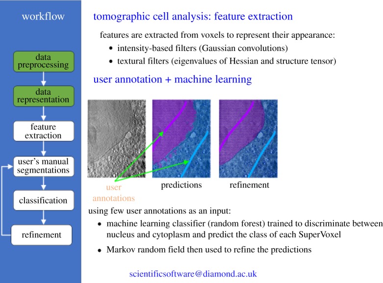
Figure 1.
A schematic of the workflow for a Cryo-Soft X-ray tomography experiment showing how user annotation of a few images can be used to train a machine learning classifier to distinguish between the cell n...
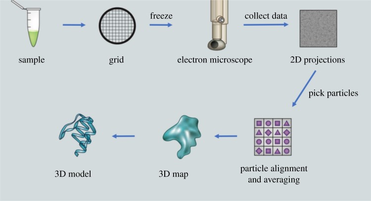
Figure 2.
A schematic of the single-particle reconstruction cryoEM pipeline. Image thanks to Creative Biostructure, https://www.creative-biostructure.com . (Online version in colour.)
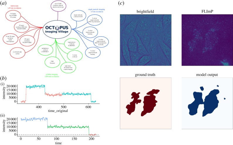
Figure 3.
( a ) Overview of the techniques employed at OCTOPUS. ( b ) An illustration of the automating FLImP integrated intensity track selection process. ( b i) Raw FLImP track showing regions deemed suitable...
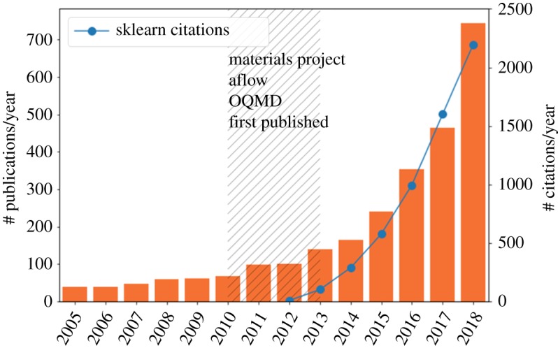
Figure 4.
The ML explosion in materials science. The number of papers containing the terms machine learning and materials are plotted on a bar chart. We indicate the dates of materials data repositories becomin...
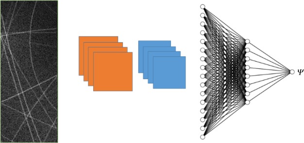
Figure 5.
A schematic of the CNN used to predict coupling azimuthal angle from DMS images. A two-dimensional map of multiple scattering lines is passed through two convolutional layers, flattened and passed thr...
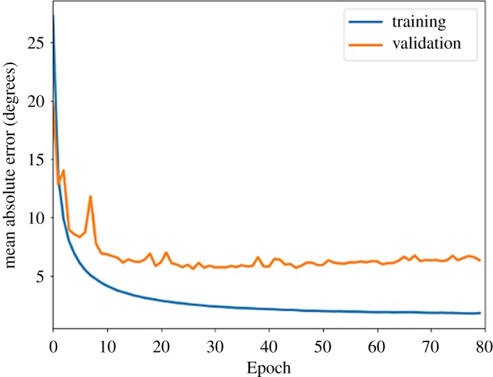
Figure 6.
Training and validation scores for the mean absolute error for the prediction of the azimuthal angle of a DMS pattern. (Online version in colour.)
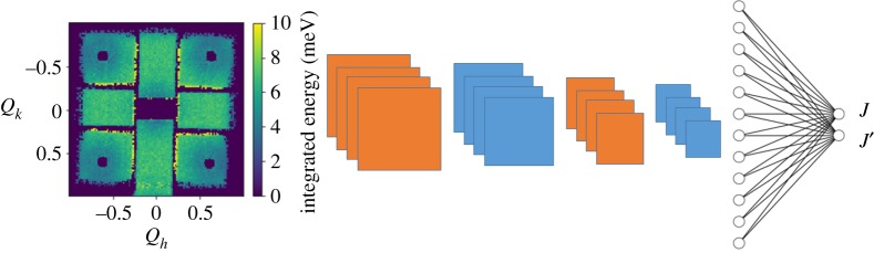
Figure 7.
A schematic of the CNN used to predict coupling constants from inelastic neutron scattering images. A two-dimensional map of integrated energy is passed through four convolutional layers, flattened an...
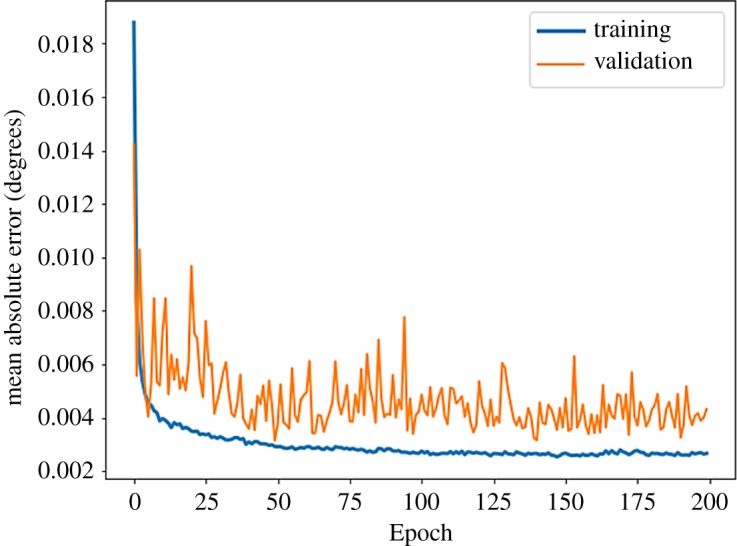
Figure 8.
Training and validation scores for the mean absolute error for the prediction of the coupling constants from an inelastic neutron scattering pattern. (Online version in colour.)
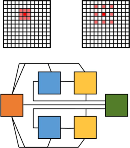
Figure 9.
Top: an illustration of a typical convolution filter (left) which convolves information from neighbour pixels and a dilation filter (right) which can convolve with pixels further removed. Lower: a sch...

Figure 10.
An example of two-dimensional scattering patterns for sub-shapes of sphere, cylinder, ellipsoid and parallelepiped shapes, from left to right. The profiles were generated by using the SASView Software...
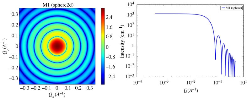
Figure 11.
An example of two-dimensional and one-dimensional scattering profile of a simple spherical particle. The profiles were generated by using the SASView Software [ 53 ]. (Online version in colour.)
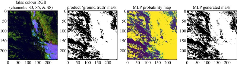
Figure 12.
This shows an example of cloud masking data. Left to right: actual image, ground truth, our generated probability mask and our generated map. Here, white regions represent the cloud and yellow regions...
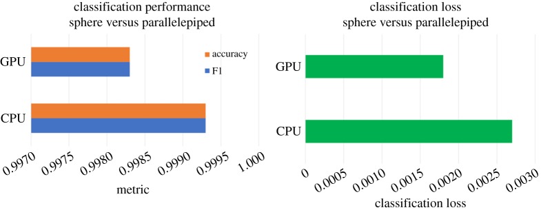
Figure 13.
Performance of the SAXS-baseline model on CPU and GPU systems. The figure shows the classification performance of the binary classification problem on the one-dimensional profiles of mono-disperse sha...
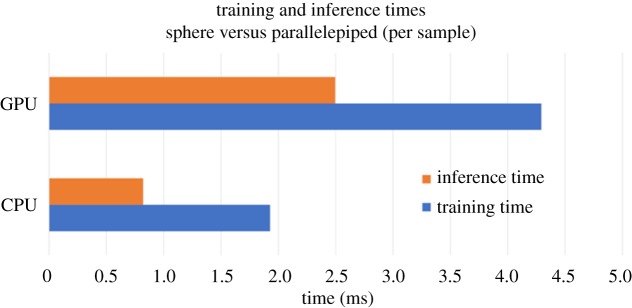
Figure 14.
Training and inference time per sample across two datasets for the SAXS-1D benchmark. (Online version in colour.)
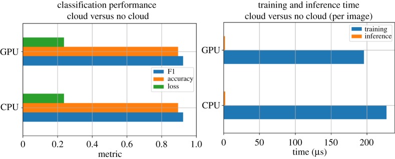
Figure 15.
Classification and runtime performance for the Sentinel-SLSTR benchmark, where the classification task is to mark each pixel as u2018cloudu2019 or u2018not cloudu2019. (Online version in colour.)
Figure images are served from the NIH/NLM PubMed Central Open Access Subset or Europe PMC; copyright remains with the publishers and authors.
💬 Discussion
0 commentsNo comments yet. Be the first to start a discussion!
Leave a Comment