Abstract
BACKGROUND: Tilt series are commonly used in electron tomography as a means of collecting three-dimensional information from two-dimensional projections. A common problem encountered is the projection alignment prior to 3D reconstruction. Current alignment techniques usually employ gold particles or image derived markers to correctly align the images. When these markers are not present, correlation between adjacent views is used to align them. However, sequential pairwise correlation is prone to bias and the resulting alignment is not always optimal. RESULTS: In this paper we introduce an algorithm to find regions of the tilt series which can be tracked within a subseries of the tilt series. These regions act as landmarks allowing the determination of the alignment parameters. We show our results with synthetic data as well as experimental cryo electron tomography. CONCLUSION: Our algorithm is able to correctly align a single-tilt tomographic series without the help of fiducial markers thanks to the detection of thousands of small image patches that can be tracked over a short number of images in the series.
🔬 Techniques
💻 Software
🧪 Sample Preparation
🏭 Microscope Brands
💻 Software Details
🏛️ Research Organizations (ROR)
Affiliated research institutions:
📋 Methods
Experimental data
For testing the algorithm with real data a tilt series of a Pyrodictium abyssi cell strain TAG11 [ 24 ], which was embedded in a vitreous ice layer [ 25 ] on a holey carbon-coated grid, was used. Electron tomography was performed using a CM120 Biofilter (FEI, Eindhoven, The Netherlands) at an accelerating voltage of 120 keV. It was equipped with a postcolumn energy filter (Gatan, Pleasanton, CA), operated in the zero-loss mode [ 26 ], resulting in increased image contrast [ 27 ]. The tilt series ranged from -70° to +67° with a tilt increment of 1.5° and a total number of 91 images. Data acquisition was carried out using fully automated procedures under low-dose conditions [ 28 ]. The images, which were 1024 × 1024 pixels each, were recorded at 14,500× magnification, with a pixel size at the specimen level of 1.62 nm. The defocus was set to -10 μ m; the first zero of the phase-contrast transfer function was at (5.8 nm) -1 . The images collected were not lowpass filtered or deconvolved with the microscope contrast transfer function. Our algorithm was run with chain lengths of 5, a correlation threshold of 0.9, local regions of a size of 4% the total size of the images (patches of size 41 × 41 pixels, with an overlap of 15 pixels). 1255 landmark chains were identified with an average length of 15.65 images. 706 landmark chains were used in the last regression iteration. There was an average error between the projection of the 3D landmarks and its observed projections of 0.85 pixels. The resulting reconstruction can be seen in Fig. 2 . For comparison purposes we performed a reconstruction from the same dataset using the standard alignment algorithm based on manual selection of fiducial markers which is shown in Fig. 3 . For the manual alignment four landmarks were identified along the whole tilt series and TOM toolbox was used for the alignment and 3D reconstruction [ 29 ]. As can be seen, the two reconstructions are not significantly different, although they are not identical. The correlation between the two volumes after registration was 0.635, however, as can be seen in Fig. 4 , these differences are not located where the archaeobacteria is and are mainly located in the surrounding structure (this is most likely due to the fact that the manually selected landmarks were chosen from the bacteria region while the surrounding objects were disregarded). Figure 2 Experimental data reconstructed automatically . Three orthogonal slices of the Pyrodictium abyssi . The three slices are shown in 3D with their relative orientations (top) as well as separately. The scalebar represents 500 nm. Figure 3 Experimental data reconstructed automatically . Top: Corresponding orthogonal slices of the volume in Fig. 2 which was reconstructed using the parameters estimated by the proposed automatic alignment algorithm. Bottom: Reconstruction of the same dataset used in Fig. 2 aligned by manually selecting the fiducial markers instead of using the automatic alignment algorithm presented in this paper. Figure 4 Slice of the difference between the two volumes shown in Fig. 3 . As can be seen most of the differences between the two volumes are not located where the bacteria is.
Show full methods section
Experimental data
For testing the algorithm with real data a tilt series of a Pyrodictium abyssi cell strain TAG11 [ 24 ], which was embedded in a vitreous ice layer [ 25 ] on a holey carbon-coated grid, was used. Electron tomography was performed using a CM120 Biofilter (FEI, Eindhoven, The Netherlands) at an accelerating voltage of 120 keV. It was equipped with a postcolumn energy filter (Gatan, Pleasanton, CA), operated in the zero-loss mode [ 26 ], resulting in increased image contrast [ 27 ]. The tilt series ranged from -70° to +67° with a tilt increment of 1.5° and a total number of 91 images. Data acquisition was carried out using fully automated procedures under low-dose conditions [ 28 ]. The images, which were 1024 × 1024 pixels each, were recorded at 14,500× magnification, with a pixel size at the specimen level of 1.62 nm. The defocus was set to -10 μ m; the first zero of the phase-contrast transfer function was at (5.8 nm) -1 . The images collected were not lowpass filtered or deconvolved with the microscope contrast transfer function. Our algorithm was run with chain lengths of 5, a correlation threshold of 0.9, local regions of a size of 4% the total size of the images (patches of size 41 × 41 pixels, with an overlap of 15 pixels). 1255 landmark chains were identified with an average length of 15.65 images. 706 landmark chains were used in the last regression iteration. There was an average error between the projection of the 3D landmarks and its observed projections of 0.85 pixels. The resulting reconstruction can be seen in Fig. 2 . For comparison purposes we performed a reconstruction from the same dataset using the standard alignment algorithm based on manual selection of fiducial markers which is shown in Fig. 3 . For the manual alignment four landmarks were identified along the whole tilt series and TOM toolbox was used for the alignment and 3D reconstruction [ 29 ]. As can be seen, the two reconstructions are not significantly different, although they are not identical. The correlation between the two volumes after registration was 0.635, however, as can be seen in Fig. 4 , these differences are not located where the archaeobacteria is and are mainly located in the surrounding structure (this is most likely due to the fact that the manually selected landmarks were chosen from the bacteria region while the surrounding objects were disregarded). Figure 2 Experimental data reconstructed automatically . Three orthogonal slices of the Pyrodictium abyssi . The three slices are shown in 3D with their relative orientations (top) as well as separately. The scalebar represents 500 nm. Figure 3 Experimental data reconstructed automatically . Top: Corresponding orthogonal slices of the volume in Fig. 2 which was reconstructed using the parameters estimated by the proposed automatic alignment algorithm. Bottom: Reconstruction of the same dataset used in Fig. 2 aligned by manually selecting the fiducial markers instead of using the automatic alignment algorithm presented in this paper. Figure 4 Slice of the difference between the two volumes shown in Fig. 3 . As can be seen most of the differences between the two volumes are not located where the bacteria is.
Methods
Affine registration of two images Given any two images I ( i ) and I ( j ) the affine registration tries to find an affine matrix (1) transforming homogeneous coordinates ( t H ) of the image i into the image j . We look for this affine transformation by maximizing the cross-correlation of the images registered bidirectionally [ 32 , 33 ] (2) The cross-correlation in each direction is carefully computed only in those regions which are visible in both images, i.e., only at those coordinates t H such that t H ∈ Ω i and A ij t H ∈ Ω j , being Ω i and Ω j the set of coordinates where the images i and j are defined. The maximization problem in Eq. 2 is solved using two different optimizers: Differential Evolution (DE) [ 34 ] and Powell's conjugate gradient method [ 35 ]. DE is a global optimizer based on genetic algorithms. It is rather good at approximately finding the best affine transformation between any two images. However, its convergence once it is closed to the global optimum is rather slow. Then we change to a fast local optimizer such as Powell's conjugate gradient method. In this way, we have the advantages of a global optimizer with a fast, locally convergent algorithm. Landmark chains In our algorithm, image regions act as landmarks. Therefore, we must track image regions along the tilt series. However, since it is rather unlikely that the same region can be tracked along the whole series, we allow for landmark chains that start at a given image of the tilt series and finish in some other image. The region being matched along the chain need not to be detectable in all images in between the first and last image. Every image in the tilt series, I ( i ) , is divided in a fine grid of overlapping image regions of a size much smaller than the whole projection. The center of each region is a landmark candidate. Given a region in image i , this region is sought in image i + 1, first by predicting its position using the affine transformation A i , i +1 computed in the previous section, and then by locally optimizing the correlation index between the two corresponding regions. If the correlation index is greater than a given threshold, then the region in image i + 1 is accepted as the one matching the landmark region in image i . The new region in image i + 1 is sought in image i + 2, and the process is subsequently repeated until the correlation threshold criterium is not met. The same procedure is performed backwards. At the end of this process we have a landmark chain extending from image i - N to image i + M for some integers N and M . If the landmark chain is shorter than a certain user-supplied threshold, the chain is discarded. If the landmark chain survives the previous filter, it is refined in an iterative way in order to avoid coordinate drifts due to the sequential search of regions. For all images between i - N + 2 and i + M the coordinate of the landmark in image l is refined with respect to that in image l - 2. This correction runs forward in the chain. When it finishes, the positions are corrected backwards (the position at image l is refined with respect to that of image l + 1) running from i + M to i - N + 1. This process is repeated with forward steps of 3, 4, ... up to a value selected by the user (i.e., the landmark at image l is refined with respect to the image l - 3, l - 4, ... respectively), while the backward correction is always performed with a step of 1. After this correction loops, the average of all regions in the chain is computed. Those regions that do not meet the correlation criterium with the average region are removed from the chain. Then the whole refinement step is repeated once again with the surviving images. Those chains whose length after refinement is smaller than the specified threshold are discarded. Optimization of the 3D landmarks and the image in-plane rotation and shift Once a list of landmark chains is produced in the previous section, each chain is assumed to correspond to the projection of the same 3D region, whose center is projected onto the center of each region. The 3D coordinates of these 3D landmarks as well as the rigid transformation parameters explaining the rotations and shifts of each projection in the tilt series are computed by robust regression. Let r j be the 3D coordinate of the j -th landmark and let p ij be the 2D coordinate of its projection onto image i . Let V j be the set of all images on which the j -th landmark is seen (remind that the landmark chain may not contain all images between i - N and i + M ). Then, the relationship between r j and p ij can be expressed as (3) where A i is a projection matrix accounting for the tilting around the tilt axis (which may have any arbitrary orientation in the plane perpendicular to the electron beam) and a posterior in-plane rotation, and d i is a 2D vector accounting for an in-plane shift of image i . A i is computed as (4) where H is a matrix projecting a 3D coordinate onto the XY plane, is a rotation matrix of ψ i degrees around the Z axis (note that the Z axis is the beam axis, therefore, this represents the in-plane rotation particular to each image), and is a rotation matrix of θ i degrees (the tilt angle of each image) around the tilt axis u axis . The tilt axis is described by two Euler angles α and β corresponding to a rotation around the Z axis and, then, a rotation around the new Y axis. The vector representation of the direction of the tilt axis is (5) Note that this projection model assumes that the tilt axis passes through the coordinate system origin. In practice this is seldom the case, although as shown later in the Appendix, the tilt axis can be arbitrarily placed in the tilt series as long as the aligned projections are consistent with the assigned position. The regression problem is to minimize the error between the projections of the 3D landmarks experimentally observed and their projections under theoretical tilting and in-plane rotation and shift (6) or what is the same (7) where V i is the set of landmarks detectable in the image i . This regression problem is linear in d i and r j and non-linear in ψ i , α and β . To find the minimizer of Eq. 7 we decompose the problem in two nested searches. The first search explores the α , β -space. For each combination of α and β proposed in a first stage by an exhaustive grid search and in a second stage by Powell's conjugate gradient method whose initial solution is the minimizer of the exhaustive grid search, the minimum is sought in the ψ i , d i and r j parameters. The minimum in these three parameters are sought in an iterative way by assuming all the rest of the parameters fixed and minimizing the goal function ( E ) with respect to the parameter treated at each time. Note that this optimization procedure may be trapped in a local minimum and that this optimization process is different from the one performed to find the affine transformation previously described. It can be easily shown (see next section) that (8) In the same way, (9) where is the average of all landmark projections in image i and is the average of all the current estimates of the 3D landmarks visible in image i . Finally (see next section), (10) and (11) Derivation of the matrix form of the regression problem In this section we derive in a compact form the minimization of the regression problem. Let E be the goal function in Eqs. 6 and 7 (12) We compute the derivatives of this goal function using the vector derivatives and . From these rules, it is easy to derive (13) being N i the number of elements of V i , i.e., the number of 3D landmarks visible in image i . From this last equation it follows (14) Now deriving with respect to r j (15) from which (16) Considering that , and given the specific nature of H and , A i can also be expressed as . We will refer to as . Then, the goal function E can be expressed as (17) Now we compute the derivative of E with respect to using the matrix derivative rule (18) Taking into account that a clockwise rotation matrix is given by , then (19) From which it can be easily derived (20) Robust optimization The optimization procedure described in the previous sections is firstly run with all landmark chains detected. Then, the fitting error is computed for each landmark chain j as (21) A user-supplied percentage of the chains with worse fitting errors are removed from the list of landmark chains assuming that they may correspond to chains that have been wrongly computed, and all the parameters (direction of the tilt axis, position of the 3D landmarks and image in-plane rotation and shifts) are reestimated with the chains remaining. This process is repeated three times, in this way a robust fitting of the alignment parameters is performed.
📊 Figures
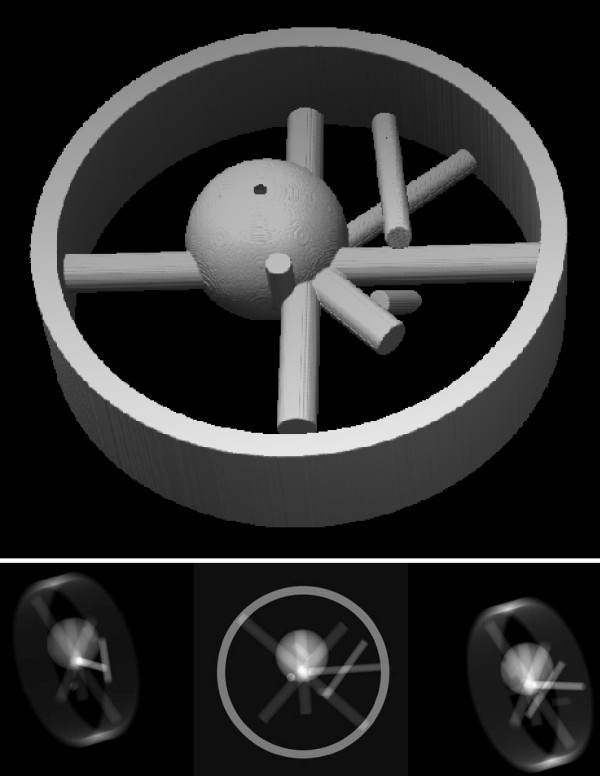
Figure 1
Phantom data . Top:Isosurface of the phantom used for the simulated data. Bottom: Projections of this phantom at -60u00b0, 0u00b0, and 60u00b0. The tilt axis forms 78u00b0 with the horizontal axis. Th...
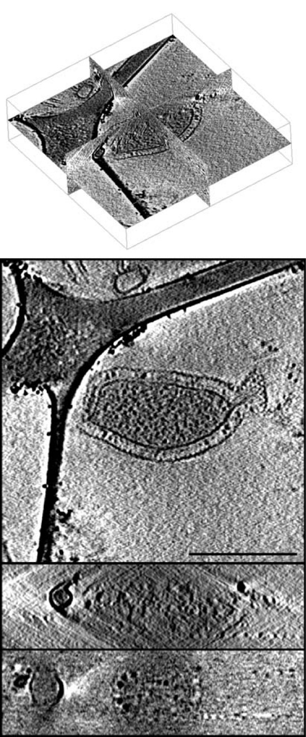
Figure 2
Experimental data reconstructed automatically . Three orthogonal slices of the Pyrodictium abyssi . The three slices are shown in 3D with their relative orientations (top) as well as separately. The s...
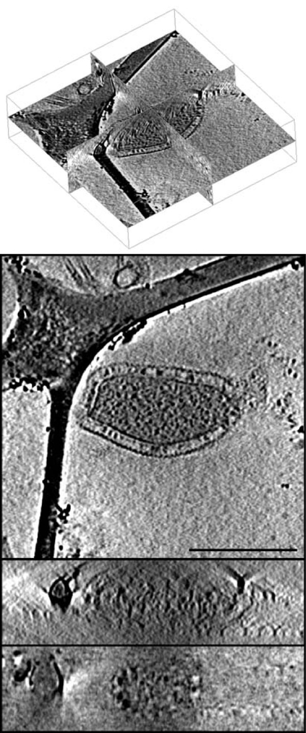
Figure 3
Experimental data reconstructed automatically . Top: Corresponding orthogonal slices of the volume in Fig. 2 which was reconstructed using the parameters estimated by the proposed automatic alignment ...

Figure 4
Slice of the difference between the two volumes shown in Fig. 3 . As can be seen most of the differences between the two volumes are not located where the bacteria is.
Figure images are served from the NIH/NLM PubMed Central Open Access Subset or Europe PMC; copyright remains with the publishers and authors.
💬 Discussion
0 commentsNo comments yet. Be the first to start a discussion!
Leave a Comment