Abstract
Most biomolecular processes rely on tightly controlled stoichiometries, from the formation of molecular assemblies to cellular signaling. Single-molecule localization microscopy studies of fluorophore blinking offer a promising route to probe oligomeric states. Here we show that the distribution of the number of blinking events assumes a universal functional form, independent of photophysics, under relatively mild assumptions. The number of photophysical states, the kinetics of interconversion, and the fraction of active fluorophores enter as two or three constants. This essentially model-independent formulation allows us to determine molecule counts from fluorophore blinking statistics. The formulas hold even if the fluorophores have many different yet unresolved dark states, as long as there is only a single fluorescent state, or if there are different yet unresolvable fluorescent states, as long as there is only a single dark state. We demonstrate the practical applicability of this approach by quantifying the oligomerization states of membrane proteins tagged with the mEos2 fluorescent protein. We find that the model parameters, obtained by likelihood maximization, are transferable. With the counting statistics being independent of the detailed photophysics and its parameters being transferable, the method should be robust and broadly applicable to counting colocalized molecules in vivo and in vitro.
🔬 Techniques
✨ Fluorophores
🧪 Sample Preparation
🏛️ Research Organizations (ROR)
Affiliated research institutions:
📋 Methods
In the following, we derive the general expression for the probability p m ( n ) of the number n of times fluorophores light up at a particular location with m + 1 colocalized fluorophores, where counting starts after the first light-up event at this location. For a single fluorophore ( m = 0), n is just the number of blinking events. If multiple fluorophores are colocalized ( m > 0), then n can be a combination of other fluorophores lighting up and of blinking events of any of the fluorophores that have already lit up at this position. By lumping together all events after the first lighting up, we account for the fact that, typically, one cannot distinguish between blinking of an already active fluorophore and a new fluorophore lighting up for the first time. We assume that all events of fluorophores lighting up are detected and resolved. We also assume that active fluorophores bleach during the observation time. Moreover, we assume either that we have only one kind of fluorophore or that different fluorophores can be distinguished, for example, by their color. The blinking statistics of colocalized fluorophores is assumed to be independent. The essence of the approach is to formulate the problem of counting in terms of transitions between microstates, which allows us to ignore the time dependence that would normally be required in kinetic modeling. We will show that the functional form of p m ( n ) is independent of the photophysics. Single fluorophore Consider a single fluorophore with multiple photophysical states i = 1,2,…, N , where the N th state is the irreversibly bleached state. We assume that the transitions between the N states are Markovian, that is, probabilistic and independent of the preceding history. Let be the probability that a molecule in state j transitions to state i directly, with . In the conventional kinetic formulation with rate coefficients k ij , one would have Our formulation accounts for all such kinetic models and more complex descriptions of the dynamics, possibly with nonexponential waiting times, albeit with Markovian transition probabilities between states. Of importance, we do not explicitly include the inactive state(s) of the fluorophore in our formulation. Instead, we deal with fluorophore activation implicitly by starting the blinking count only after activation of a first fluorophore and lumping the activation of additional colocalized fluorophores together with the (indistinguishable) blinking events of already active fluorophores. Now let transitions from state j = d to state i = f correspond to the blinking event of interest, with state d being dark and state f fluorescent. To determine the probability p 0 ( n ) of the number of times n such a transition occurs before eventual bleaching starting from a particular state k , we use a generating-function formulation ( Bicout and Rubin, 1999 ; Brown, 2003 ; Gopich and Szabo, 2003 ). We define a modified transition matrix T ( z ) whose elements are T ij , except for the ( f , d ) element, which is multiplied by z , With 0 ≤ z ≤ 1, we can think of T ( z ) as a transition matrix with an additional irreversible process: whenever the system is in state d , there is a nonzero probability of “dying,” since for 0 ≤ z < 1. For a transition trajectory starting in state k and evolving according to T ( z ), we define w k ( z ) as the probability of reaching the bleached state N instead of dying along the way in state d . This probability is the generating function for the transition counts, ( 1 ) This key relation is usually derived using Laplace transforms for specific dynamics ( Bicout and Rubin, 1999 ; Brown, 2003 ; Gopich and Szabo, 2003 ). Here, for our transition dynamics, it follows immediately from the expression of the overall probability of going from state k to state N in M transitions according to the modified transition matrix In this path integral (or, more appropriately, path sum) representation of the propagator, evaluated conveniently as the ( N , k ) element of the M th power of T ( z ) and then represented as a power series in z , the coefficient of z n is exactly the combined contribution to the overall k → N transition probability for the unmodified dynamics (i.e., for z = 1) of all paths in which the transition d → f has occurred exactly n times. By definition, the generating function w k ( z ) is identical to the so-called committor (or splitting) probability. We assume that any fluorophore lighting up eventually bleaches, here by reaching state N , which allows us to take the limit of infinitely many transitions, M → ∞. Then, by the conservation of probability, With w N ( z ) = 1 by definition, we thus arrived at the usual expression for the committor in terms of the adjoint of the evolution operator ( Onsager, 1938 ; here the transpose of T ( z )). Therefore the vector w ( z ) of the N − 1 probabilities w 1 ( z ),..., w N -1 ( z ) of reaching state N without dying in the special state d satisfies ( 2 ) where is an ( N − 1) × ( N − 1) matrix of elements ( 3 ) for 1 ≤ i , j ≤ N − 1 (i.e., excluding the bleached state N ). is thus the transpose of the first N − 1 rows and columns of T ( z ) minus the identity matrix, the Kronecker being 1 for i = j and 0 otherwise. The vector t has elements ( 4 ) for i = 1 to N − 1 and is thus independent of z . We note in passing that identical expressions for w ( z ) are obtained if one takes the infinite-transition limit, evaluating explicitly in a spectral expansion, or by using the fact that P ( z ) is a projector that satisfies . To derive the most general functional form of the generating functions w k ( z ), we express the matrix inverse in Eq. 2 in terms of determinants, denoted as |…|. We have , where matrix constructed by deleting row i and column j in From the definition of determinants as sums over all signed permutations of the matrix coefficients, it follows that w k ( z ) is a rational function of z in which the denominator is linear in z and the numerator is either constant (independent of z ) or linear in z . Here we exploited the fact that only the ( f , d ) element of T depends on z . We thus arrive at the most general form of the generating function, ( 5 ) where we added a superscript “(0)” to indicate that we have a single fluorophore and took advantage of the fact that the conservation of probability requires w k ( z = 1) = 1. In Eq. 5, we averaged over the initial states k . After photoactivation, we assume the fluorophore to be in one of the fluorescent states k with probability π k (with π k = 0 for nonfluorescent states), such that is a weighted average over the generating functions for the blinking counts starting in state k . Changing the probabilities π k can alter the value of w (0) ( z ) but not the form of p 0 . The parameters p and p 0 in Eq. 5 are sums of products of the transition probabilities T ij and thus reflect the photophysics of the fluorophore, as illustrated later by specific examples. The functional form Eq. 5 of w (0) ( z ) corresponds to a renewal process ( Cao and Silbey, 2008 ) in two steps, or in one step if p = p 0 . We note that explicit expressions for w k ( z ) can be derived using the Sherman–Morrison formula for matrix inverses. Because, by definition, the two parameters are themselves probabilities, (see also Eq. 9 later). As we will show later, for simple fluorophores with single dark and fluorescent states, we have p = p 0 and thus a z -independent numerator as a further simplification. Multiple colocalized fluorophores When multiple fluorophores are colocalized, an observed blinking event can be caused either by blinking of an already active fluorophore or by a previously inactive fluorophore lighting up for the first time. The generating function of the probability p m ( n ) of counting n uncorrelated events for m + 1 colocalized fluorophores is thus ( 6 ) where the first w (0) ( z ) accounts for the first fluorophore to light up. The second term accounts for the remaining m fluorophores. In this term, w (0) ( z ) is thus multiplied by z because lighting up is counted as an event that, we assume, cannot be distinguished from blinking. (Note that in the generating-function formalism, multiplying by z amounts to increasing the count by 1, and multiplying generating functions assumes that counts of the factors—here of the m + 1 colocalized fluorophores—are statistically independent.) The initial activation of a fluorophore during the observation time is weighted by the probability 1 − q , where q is the fraction of fluorophores that do not light up during the observation time, in particular due to incomplete assembly or damage other than eventual photobleaching. By combining Eqs. 5 and 6, we arrive at the most general form of the generating function. By using the definition of the generating function, , the binomial theorem , and the geometric series we obtain the general expression for the probability p m ( n ) of n counts, given m + 1 colocalized identical fluorophores, ( 7 ) where is the binomial coefficient and ( 8 ) For m = 0 specifically, we obtain ( 9 ) In a computer, the probabilities p m ( n ) can be conveniently evaluated by recursion: ( 10 ) starting from Eq. 9, and . This recursion formula was obtained from Eq. 6 by matching the coefficients of z n . Simple fluorophores If p 0 = p , the count probability simplifies to ( 11 ) expressed compactly in terms of a hypergeometric function. For m = 0, 1, and 2 and we obtain ( 12 ) ( 13 ) ( 14 ) Note that for simple fluorophores in the limit of q → 0 (i.e., all fluorophores are active), we recover the negative binomial distribution derived previously by Lee et al. (2012) using kinetic modeling, albeit with one difference. Because we count the initial light-up of a fluorophore as an event, the distribution p m ( n ) here is shifted to larger n values by exactly m , that is, p m ( n − m ) for q = 0 is the negative binomial distribution. Mean and variance From the k th derivative of the generating function with respect to z evaluated at z = 1, we obtain the factorial moments of the number of counts n for m + 1 colocalized fluorophores as The mean number of counts is ( 15 ) reducing to for the special case of p = p 0 . For the variance of n , we find ( 16 ) which reduces to for p = p 0 . Simple fluorophore To illustrate how photophysics determines the model parameters p and p 0 , we first consider the simplest case of a fluorophore with three states ( i = 1, 2, 3): D (dark), F (fluorescent), and B (bleached). In this model, bleaching occurs only from the fluorescent state and is irreversible. The nonzero elements of the modified transition matrix are T 12 = 1 − p , T 21 ( z ) = z , T 32 = p , and T 33 = 1, where p is the probability of bleaching from the fluorescent state. From Eq. 2, we obtain the generating function for a single active fluorophore that is, we have the special case of p 0 = p . Accordingly, the blinking statistics for m + 1 colocalized fluorophores follows p m ( n ) in Eq. 11. To account for the possibility that bleaching occurs also from the dark state, D → B, with a probability r , we set T 21 ( z ) = z (1 − r ) and T 31 = r . The generating function, where u = p (1 − r ) + r , thus falls again into the simple one-parameter category. However, the interpretation of the single coefficient (now u instead of p !) has changed, since u is a combination of the probabilities p and r of bleaching in the fluorescent and dark states, respectively. Two fluorescent states In the case of two fluorescent states in series, the modified transition matrix has nonzero elements T 12 = 1 − r , T 21 ( z ) = z , T 23 = 1 − p , T 32 = r , T 43 = p , and T 44 = 1, where r is the probability of transitioning from F 1 to F 2 , and p is the probability of bleaching from the fluorescent state F 2 . For simplicity, we assume that after photoactivation, we have an equilibrium of F 1 and F 2 states. The generating function for the number of blinking events starting from F 1 or F 2 according to this equilibrium assumes the general form with and . In this case, the counting statistics for m + 1 fluorophores adopts the more complex form of Eq. 7 with instead of p . Two dark states We also considered the case of two dark states, D 1 and D 2 , and one fluorescent state F, a model that was found to describe the photophysics of two popular photoactivatable fluorescent proteins in SMLM, Dendra2 and mEos2 ( Lee et al. , 2012 ). For the sake of generality, we allowed all states to interconvert into each other in principle and to photobleach. The resulting transition matrix T is thus dense. Nonetheless, the generating function w (0) ( z ) of the blinking counts starting from the F state assumes the simple form of Eq. 11 for p = p 0 . However, in this most general case, the coefficients p = p 0 are relatively complicated sums of products of the transition matrix elements. Indistinguishable blinking transitions A possible complication arises if different transitions d i → f i ( i = 1,2,…) between distinct dark states d i and fluorescent states f i result in blinking but cannot be distinguished. To lump together the counts of all d i → f i transitions, we multiply all corresponding elements in the transition matrix with z , , and then determine the generating functions w k ( z ) using Eq. 2. If the transitions i share either a common fluorescent state ( f 1 = f 2 = ...) or a common dark state ( d 1 = d 2 = ...), all z -containing elements will be in a row or a column of T ( z ), respectively (as, e.g., in the preceding example of two fluorescent states). Following the foregoing derivation and once more invoking the definition of determinants, one finds that the generating function again takes Eq. 5 as its most general form, irrespective of having lumped together counts for different transitions d i → f i . By contrast, if neither the fluorescent nor the dark states are common, the generating functions w k ( z ) for the probability of the number n of transitions will still be a rational function of z . However, the order of the z -polynomials in the numerator and denominator can be higher than linear. Note that if the different transitions i can be distinguished, then we can use the generating-function approach to calculate the joint probabilities p ( n 1 , n 2 ,...) of seeing i = 1, n 2 transitions of type i = 1, n 2 transitions of type 2, and so on in the same trace. If the respective transition matrix elements are multiplied by , and w k is constructed as above, then the coefficient of the ... term in the series expansion of w k ( z 1 , z 2 ...) is the joint probability. From experiment to molecule counts The explicit expressions for the count probabilities p m ( n ) in Eqs. 7 and 11 make it possible to use likelihood-based approaches to decide between the simple case of p = p 0 and the more complex case and infer the unknown parameters ( p , p 0 , q , and m ) from the observed blinking statistics. We define c ( n ) as the number of spots at which exactly n blinking events have been counted, with the total number of spots analyzed. c ( n ) is thus the frequency distribution of an integer number of blinking counts, whose construction does not require binning of a continuous variable. For uncorrelated events and only counting noise, the log-likelihood function is ( 17 ) In a maximum-likelihood approach, L is maximized with respect to the parameters entering p m ( n ). Alternatively, in a Bayesian formulation, we could use priors on the parameters that reflect our expectations on these parameters and use L to define the posterior. In the simple case of p = p 0 for a single fluorophore, m = 0, maximization of L with respect to p results in . In the general case with and m = 0, L is maximal for and . The maximum-likelihood solution for q , with m > 0, has to be determined numerically, for example, by Newton–Raphson iteration or bisection. According to the BIC, the log-likelihood L should increase by at least to justify the more complex model, Eq. 7 with , over the simple model, Eq. 11. Unresolved events If blinking events are fast, not all of them may be resolved. A simple way to account for missed events is to assume that events are resolved with probability r and missed with probability 1 − r . The observed distribution is then ( 18 ) The k th factorial moments of the observed and actual numbers of counts are related by . In a further extension of this formulation, one could introduce also false positives that arise, for example, from contaminations. If these are not treated properly, a few large n might have an undue influence on the results. Our approach is compatible with overlapping blinking cycles. However, if more than one molecule lights up at the same time in a particular spot, this may be detected as only one blinking event, leading to underestimation of n . We expect this scenario to be extremely rare even at higher molecular densities; it can be circumvented by adjusting the experimental activation settings such that only low densities of molecules light up.
Show full methods section
In the following, we derive the general expression for the probability p m ( n ) of the number n of times fluorophores light up at a particular location with m + 1 colocalized fluorophores, where counting starts after the first light-up event at this location. For a single fluorophore ( m = 0), n is just the number of blinking events. If multiple fluorophores are colocalized ( m > 0), then n can be a combination of other fluorophores lighting up and of blinking events of any of the fluorophores that have already lit up at this position. By lumping together all events after the first lighting up, we account for the fact that, typically, one cannot distinguish between blinking of an already active fluorophore and a new fluorophore lighting up for the first time. We assume that all events of fluorophores lighting up are detected and resolved. We also assume that active fluorophores bleach during the observation time. Moreover, we assume either that we have only one kind of fluorophore or that different fluorophores can be distinguished, for example, by their color. The blinking statistics of colocalized fluorophores is assumed to be independent. The essence of the approach is to formulate the problem of counting in terms of transitions between microstates, which allows us to ignore the time dependence that would normally be required in kinetic modeling. We will show that the functional form of p m ( n ) is independent of the photophysics. Single fluorophore Consider a single fluorophore with multiple photophysical states i = 1,2,…, N , where the N th state is the irreversibly bleached state. We assume that the transitions between the N states are Markovian, that is, probabilistic and independent of the preceding history. Let be the probability that a molecule in state j transitions to state i directly, with . In the conventional kinetic formulation with rate coefficients k ij , one would have Our formulation accounts for all such kinetic models and more complex descriptions of the dynamics, possibly with nonexponential waiting times, albeit with Markovian transition probabilities between states. Of importance, we do not explicitly include the inactive state(s) of the fluorophore in our formulation. Instead, we deal with fluorophore activation implicitly by starting the blinking count only after activation of a first fluorophore and lumping the activation of additional colocalized fluorophores together with the (indistinguishable) blinking events of already active fluorophores. Now let transitions from state j = d to state i = f correspond to the blinking event of interest, with state d being dark and state f fluorescent. To determine the probability p 0 ( n ) of the number of times n such a transition occurs before eventual bleaching starting from a particular state k , we use a generating-function formulation ( Bicout and Rubin, 1999 ; Brown, 2003 ; Gopich and Szabo, 2003 ). We define a modified transition matrix T ( z ) whose elements are T ij , except for the ( f , d ) element, which is multiplied by z , With 0 ≤ z ≤ 1, we can think of T ( z ) as a transition matrix with an additional irreversible process: whenever the system is in state d , there is a nonzero probability of “dying,” since for 0 ≤ z < 1. For a transition trajectory starting in state k and evolving according to T ( z ), we define w k ( z ) as the probability of reaching the bleached state N instead of dying along the way in state d . This probability is the generating function for the transition counts, ( 1 ) This key relation is usually derived using Laplace transforms for specific dynamics ( Bicout and Rubin, 1999 ; Brown, 2003 ; Gopich and Szabo, 2003 ). Here, for our transition dynamics, it follows immediately from the expression of the overall probability of going from state k to state N in M transitions according to the modified transition matrix In this path integral (or, more appropriately, path sum) representation of the propagator, evaluated conveniently as the ( N , k ) element of the M th power of T ( z ) and then represented as a power series in z , the coefficient of z n is exactly the combined contribution to the overall k → N transition probability for the unmodified dynamics (i.e., for z = 1) of all paths in which the transition d → f has occurred exactly n times. By definition, the generating function w k ( z ) is identical to the so-called committor (or splitting) probability. We assume that any fluorophore lighting up eventually bleaches, here by reaching state N , which allows us to take the limit of infinitely many transitions, M → ∞. Then, by the conservation of probability, With w N ( z ) = 1 by definition, we thus arrived at the usual expression for the committor in terms of the adjoint of the evolution operator ( Onsager, 1938 ; here the transpose of T ( z )). Therefore the vector w ( z ) of the N − 1 probabilities w 1 ( z ),..., w N -1 ( z ) of reaching state N without dying in the special state d satisfies ( 2 ) where is an ( N − 1) × ( N − 1) matrix of elements ( 3 ) for 1 ≤ i , j ≤ N − 1 (i.e., excluding the bleached state N ). is thus the transpose of the first N − 1 rows and columns of T ( z ) minus the identity matrix, the Kronecker being 1 for i = j and 0 otherwise. The vector t has elements ( 4 ) for i = 1 to N − 1 and is thus independent of z . We note in passing that identical expressions for w ( z ) are obtained if one takes the infinite-transition limit, evaluating explicitly in a spectral expansion, or by using the fact that P ( z ) is a projector that satisfies . To derive the most general functional form of the generating functions w k ( z ), we express the matrix inverse in Eq. 2 in terms of determinants, denoted as |…|. We have , where matrix constructed by deleting row i and column j in From the definition of determinants as sums over all signed permutations of the matrix coefficients, it follows that w k ( z ) is a rational function of z in which the denominator is linear in z and the numerator is either constant (independent of z ) or linear in z . Here we exploited the fact that only the ( f , d ) element of T depends on z . We thus arrive at the most general form of the generating function, ( 5 ) where we added a superscript “(0)” to indicate that we have a single fluorophore and took advantage of the fact that the conservation of probability requires w k ( z = 1) = 1. In Eq. 5, we averaged over the initial states k . After photoactivation, we assume the fluorophore to be in one of the fluorescent states k with probability π k (with π k = 0 for nonfluorescent states), such that is a weighted average over the generating functions for the blinking counts starting in state k . Changing the probabilities π k can alter the value of w (0) ( z ) but not the form of p 0 . The parameters p and p 0 in Eq. 5 are sums of products of the transition probabilities T ij and thus reflect the photophysics of the fluorophore, as illustrated later by specific examples. The functional form Eq. 5 of w (0) ( z ) corresponds to a renewal process ( Cao and Silbey, 2008 ) in two steps, or in one step if p = p 0 . We note that explicit expressions for w k ( z ) can be derived using the Sherman–Morrison formula for matrix inverses. Because, by definition, the two parameters are themselves probabilities, (see also Eq. 9 later). As we will show later, for simple fluorophores with single dark and fluorescent states, we have p = p 0 and thus a z -independent numerator as a further simplification. Multiple colocalized fluorophores When multiple fluorophores are colocalized, an observed blinking event can be caused either by blinking of an already active fluorophore or by a previously inactive fluorophore lighting up for the first time. The generating function of the probability p m ( n ) of counting n uncorrelated events for m + 1 colocalized fluorophores is thus ( 6 ) where the first w (0) ( z ) accounts for the first fluorophore to light up. The second term accounts for the remaining m fluorophores. In this term, w (0) ( z ) is thus multiplied by z because lighting up is counted as an event that, we assume, cannot be distinguished from blinking. (Note that in the generating-function formalism, multiplying by z amounts to increasing the count by 1, and multiplying generating functions assumes that counts of the factors—here of the m + 1 colocalized fluorophores—are statistically independent.) The initial activation of a fluorophore during the observation time is weighted by the probability 1 − q , where q is the fraction of fluorophores that do not light up during the observation time, in particular due to incomplete assembly or damage other than eventual photobleaching. By combining Eqs. 5 and 6, we arrive at the most general form of the generating function. By using the definition of the generating function, , the binomial theorem , and the geometric series we obtain the general expression for the probability p m ( n ) of n counts, given m + 1 colocalized identical fluorophores, ( 7 ) where is the binomial coefficient and ( 8 ) For m = 0 specifically, we obtain ( 9 ) In a computer, the probabilities p m ( n ) can be conveniently evaluated by recursion: ( 10 ) starting from Eq. 9, and . This recursion formula was obtained from Eq. 6 by matching the coefficients of z n . Simple fluorophores If p 0 = p , the count probability simplifies to ( 11 ) expressed compactly in terms of a hypergeometric function. For m = 0, 1, and 2 and we obtain ( 12 ) ( 13 ) ( 14 ) Note that for simple fluorophores in the limit of q → 0 (i.e., all fluorophores are active), we recover the negative binomial distribution derived previously by Lee et al. (2012) using kinetic modeling, albeit with one difference. Because we count the initial light-up of a fluorophore as an event, the distribution p m ( n ) here is shifted to larger n values by exactly m , that is, p m ( n − m ) for q = 0 is the negative binomial distribution. Mean and variance From the k th derivative of the generating function with respect to z evaluated at z = 1, we obtain the factorial moments of the number of counts n for m + 1 colocalized fluorophores as The mean number of counts is ( 15 ) reducing to for the special case of p = p 0 . For the variance of n , we find ( 16 ) which reduces to for p = p 0 . Simple fluorophore To illustrate how photophysics determines the model parameters p and p 0 , we first consider the simplest case of a fluorophore with three states ( i = 1, 2, 3): D (dark), F (fluorescent), and B (bleached). In this model, bleaching occurs only from the fluorescent state and is irreversible. The nonzero elements of the modified transition matrix are T 12 = 1 − p , T 21 ( z ) = z , T 32 = p , and T 33 = 1, where p is the probability of bleaching from the fluorescent state. From Eq. 2, we obtain the generating function for a single active fluorophore that is, we have the special case of p 0 = p . Accordingly, the blinking statistics for m + 1 colocalized fluorophores follows p m ( n ) in Eq. 11. To account for the possibility that bleaching occurs also from the dark state, D → B, with a probability r , we set T 21 ( z ) = z (1 − r ) and T 31 = r . The generating function, where u = p (1 − r ) + r , thus falls again into the simple one-parameter category. However, the interpretation of the single coefficient (now u instead of p !) has changed, since u is a combination of the probabilities p and r of bleaching in the fluorescent and dark states, respectively. Two fluorescent states In the case of two fluorescent states in series, the modified transition matrix has nonzero elements T 12 = 1 − r , T 21 ( z ) = z , T 23 = 1 − p , T 32 = r , T 43 = p , and T 44 = 1, where r is the probability of transitioning from F 1 to F 2 , and p is the probability of bleaching from the fluorescent state F 2 . For simplicity, we assume that after photoactivation, we have an equilibrium of F 1 and F 2 states. The generating function for the number of blinking events starting from F 1 or F 2 according to this equilibrium assumes the general form with and . In this case, the counting statistics for m + 1 fluorophores adopts the more complex form of Eq. 7 with instead of p . Two dark states We also considered the case of two dark states, D 1 and D 2 , and one fluorescent state F, a model that was found to describe the photophysics of two popular photoactivatable fluorescent proteins in SMLM, Dendra2 and mEos2 ( Lee et al. , 2012 ). For the sake of generality, we allowed all states to interconvert into each other in principle and to photobleach. The resulting transition matrix T is thus dense. Nonetheless, the generating function w (0) ( z ) of the blinking counts starting from the F state assumes the simple form of Eq. 11 for p = p 0 . However, in this most general case, the coefficients p = p 0 are relatively complicated sums of products of the transition matrix elements. Indistinguishable blinking transitions A possible complication arises if different transitions d i → f i ( i = 1,2,…) between distinct dark states d i and fluorescent states f i result in blinking but cannot be distinguished. To lump together the counts of all d i → f i transitions, we multiply all corresponding elements in the transition matrix with z , , and then determine the generating functions w k ( z ) using Eq. 2. If the transitions i share either a common fluorescent state ( f 1 = f 2 = ...) or a common dark state ( d 1 = d 2 = ...), all z -containing elements will be in a row or a column of T ( z ), respectively (as, e.g., in the preceding example of two fluorescent states). Following the foregoing derivation and once more invoking the definition of determinants, one finds that the generating function again takes Eq. 5 as its most general form, irrespective of having lumped together counts for different transitions d i → f i . By contrast, if neither the fluorescent nor the dark states are common, the generating functions w k ( z ) for the probability of the number n of transitions will still be a rational function of z . However, the order of the z -polynomials in the numerator and denominator can be higher than linear. Note that if the different transitions i can be distinguished, then we can use the generating-function approach to calculate the joint probabilities p ( n 1 , n 2 ,...) of seeing i = 1, n 2 transitions of type i = 1, n 2 transitions of type 2, and so on in the same trace. If the respective transition matrix elements are multiplied by , and w k is constructed as above, then the coefficient of the ... term in the series expansion of w k ( z 1 , z 2 ...) is the joint probability. From experiment to molecule counts The explicit expressions for the count probabilities p m ( n ) in Eqs. 7 and 11 make it possible to use likelihood-based approaches to decide between the simple case of p = p 0 and the more complex case and infer the unknown parameters ( p , p 0 , q , and m ) from the observed blinking statistics. We define c ( n ) as the number of spots at which exactly n blinking events have been counted, with the total number of spots analyzed. c ( n ) is thus the frequency distribution of an integer number of blinking counts, whose construction does not require binning of a continuous variable. For uncorrelated events and only counting noise, the log-likelihood function is ( 17 ) In a maximum-likelihood approach, L is maximized with respect to the parameters entering p m ( n ). Alternatively, in a Bayesian formulation, we could use priors on the parameters that reflect our expectations on these parameters and use L to define the posterior. In the simple case of p = p 0 for a single fluorophore, m = 0, maximization of L with respect to p results in . In the general case with and m = 0, L is maximal for and . The maximum-likelihood solution for q , with m > 0, has to be determined numerically, for example, by Newton–Raphson iteration or bisection. According to the BIC, the log-likelihood L should increase by at least to justify the more complex model, Eq. 7 with , over the simple model, Eq. 11. Unresolved events If blinking events are fast, not all of them may be resolved. A simple way to account for missed events is to assume that events are resolved with probability r and missed with probability 1 − r . The observed distribution is then ( 18 ) The k th factorial moments of the observed and actual numbers of counts are related by . In a further extension of this formulation, one could introduce also false positives that arise, for example, from contaminations. If these are not treated properly, a few large n might have an undue influence on the results. Our approach is compatible with overlapping blinking cycles. However, if more than one molecule lights up at the same time in a particular spot, this may be detected as only one blinking event, leading to underestimation of n . We expect this scenario to be extremely rare even at higher molecular densities; it can be circumvented by adjusting the experimental activation settings such that only low densities of molecules light up.
📊 Figures
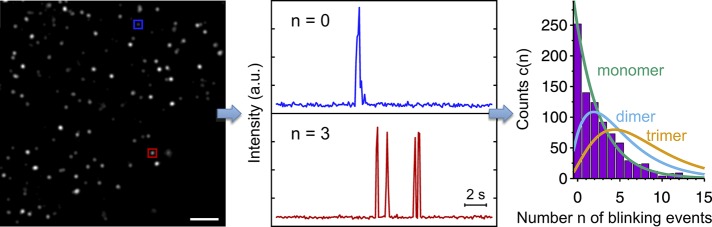
FIGURE 1:
Molecule counting in single-molecule localization microscopy. From the time-ordered series of total internal reflection images used to create the SMLM image (left; scale bar, 500 nm), one determines f...
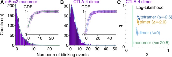
FIGURE 2:
Extraction of photophysical parameters from blinking statistics of (A) mEos2 monomers and (B, C) CTLA-4 dimers. The measured counts ( Fricke etu00a0al. , 2015a ) c ( n ) are shown as boxes. (A) For th...
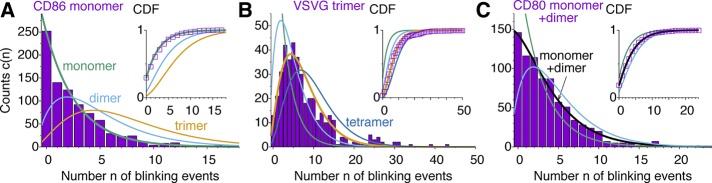
FIGURE 3:
Blinking statistics of (A) CD86-mEos2, (B) VSVG-mEos2, and (C) CD80-mEos2. Boxes show experimental counts ( Fricke etu00a0al. , 2015a ). Lines show the predicted statistics for monomers (green), dimer...
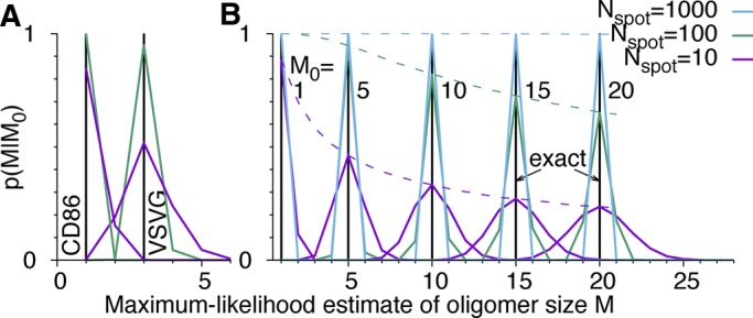
FIGURE 4:
Accuracy of estimated molecule counts M for different oligomer sizes M 0 and numbers of spots N spot analyzed. p ( M / M 0 ) is the distribution of M = m + 1 maximizing the likelihood (Eq. 17) in 10 5...
Figure images are served from the NIH/NLM PubMed Central Open Access Subset or Europe PMC; copyright remains with the publishers and authors.
💬 Discussion
0 commentsNo comments yet. Be the first to start a discussion!
Leave a Comment