Abstract
AbstractCa2+ influx triggers the release of synaptic vesicles at the presynaptic active zone (AZ). A quantitative characterization of presynaptic Ca2+ signaling is critical for understanding synaptic transmission. However, this has remained challenging to establish at the required resolution. Here, we employ confocal and stimulated emission depletion (STED) microscopy to quantify the number (20–330) and arrangement (mostly linear 70 nm × 100–600 nm clusters) of Ca2+ channels at AZs of mouse cochlear inner hair cells (IHCs). Establishing STED Ca2+ imaging, we analyze presynaptic Ca2+ signals at the nanometer scale and find confined elongated Ca2+ domains at normal IHC AZs, whereas Ca2+ domains are spatially spread out at the AZs of bassoon-deficient IHCs. Performing 2D-STED fluorescence lifetime analysis, we arrive at estimates of the Ca2+ concentrations at stimulated IHC AZs of on average 25 µM. We propose that IHCs form bassoon-dependent presynaptic Ca2+-channel clusters of similar density but scalable length, thereby varying the number of Ca2+ channels amongst individual AZs.
🔬 Techniques
🧬 Organisms
💻 Software
✨ Fluorophores
🧪 Sample Preparation
🔬 Cell Lines
🏭 Microscope Brands
🧪 Reagent Suppliers
📷 Detectors
💻 Software Details
🏛️ Research Organizations (ROR)
Affiliated research institutions:
📋 Methods
Animals
C57B6/N mice and mice carrying a deletion of exons 4 and 5 of the bassoon gene ( Bsn Δ Ex4/5 ) 38 were used at the age of postnatal day 26 (P26) to P33 (for optical fluctuation analysis) or P15 to P18 (for all other experiments). Both male and female mice were used. All experiments complied with German national animal care guidelines and the guidelines issued by the University Medical Center Göttingen.
Immunohistochemistry
Freshly dissected apical cochlear turns were fixed in methanol for 20 min at −20 °C. Thereafter, the tissue was washed three times for 10 min in PBS and incubated for 1 h in goat serum dilution buffer (GSDB) (16% normal goat serum, 450 mM NaCl, 0.3% Triton X-100, and 20 mM phosphate buffer, pH 7.4) in a wet chamber at room temperature. Primary antibodies were diluted in GSDB and applied overnight at 4 °C in a wet chamber. After washing three times for 10 min (wash buffer: 450 mM NaCl, 20 mM phosphate buffer, and 0.3% Triton X-100), the tissue was incubated with secondary antibodies in GSDB in a wet light-protected chamber for 1 h at room temperature. Then, the preparations were washed three times for 10 min in wash buffer and one time for 10 min in 5 mM phosphate buffer, placed onto the glass microscope slides with a drop of fluorescence mounting medium (Mowiol), and covered with thin glass coverslips. The following antibodies were used: mouse anti-Sap7f407 to bassoon (1:600, Abcam ab82958), rabbit anti-Ca V 1.3 (1:75, Alomone Labs ACC-005), STAR 580-tagged goat-anti-rabbit or goat-anti-mouse (1:200, Abberior 2-0002-005-1 or 2-0012-005-8), and STAR 635P-tagged goat-anti-mouse or goat-anti-rabbit (1:200, Abberior 2-0002-007-5 or 2-0012-007-2). 2D- and 3D-STED immunofluorescence images were acquired on an Abberior Instruments Expert Line 775 nm 2-color STED microscope, with excitation lasers at 561 nm and 633 nm and a STED laser at 775 nm, 1.2 W, using a 1.4 NA 100× oil immersion objective. Images were acquired with pixel sizes of 20 × 20 nm (2D-STED) or 40 × 40 × 40 nm (3D-STED). Volumetric display of 3D stacks was performed using the software Imaris (Bitplane, Zurich, Switzerland). Images were analyzed using Igor Pro 6 software (Wavemetrics, Lake Oswego, OR, USA).
Show full methods section
Animals
C57B6/N mice and mice carrying a deletion of exons 4 and 5 of the bassoon gene ( Bsn Δ Ex4/5 ) 38 were used at the age of postnatal day 26 (P26) to P33 (for optical fluctuation analysis) or P15 to P18 (for all other experiments). Both male and female mice were used. All experiments complied with German national animal care guidelines and the guidelines issued by the University Medical Center Göttingen.
Immunohistochemistry
Freshly dissected apical cochlear turns were fixed in methanol for 20 min at −20 °C. Thereafter, the tissue was washed three times for 10 min in PBS and incubated for 1 h in goat serum dilution buffer (GSDB) (16% normal goat serum, 450 mM NaCl, 0.3% Triton X-100, and 20 mM phosphate buffer, pH 7.4) in a wet chamber at room temperature. Primary antibodies were diluted in GSDB and applied overnight at 4 °C in a wet chamber. After washing three times for 10 min (wash buffer: 450 mM NaCl, 20 mM phosphate buffer, and 0.3% Triton X-100), the tissue was incubated with secondary antibodies in GSDB in a wet light-protected chamber for 1 h at room temperature. Then, the preparations were washed three times for 10 min in wash buffer and one time for 10 min in 5 mM phosphate buffer, placed onto the glass microscope slides with a drop of fluorescence mounting medium (Mowiol), and covered with thin glass coverslips. The following antibodies were used: mouse anti-Sap7f407 to bassoon (1:600, Abcam ab82958), rabbit anti-Ca V 1.3 (1:75, Alomone Labs ACC-005), STAR 580-tagged goat-anti-rabbit or goat-anti-mouse (1:200, Abberior 2-0002-005-1 or 2-0012-005-8), and STAR 635P-tagged goat-anti-mouse or goat-anti-rabbit (1:200, Abberior 2-0002-007-5 or 2-0012-007-2). 2D- and 3D-STED immunofluorescence images were acquired on an Abberior Instruments Expert Line 775 nm 2-color STED microscope, with excitation lasers at 561 nm and 633 nm and a STED laser at 775 nm, 1.2 W, using a 1.4 NA 100× oil immersion objective. Images were acquired with pixel sizes of 20 × 20 nm (2D-STED) or 40 × 40 × 40 nm (3D-STED). Volumetric display of 3D stacks was performed using the software Imaris (Bitplane, Zurich, Switzerland). Images were analyzed using Igor Pro 6 software (Wavemetrics, Lake Oswego, OR, USA).
Patch-clamp recordings
IHCs from apical coils of freshly dissected organs of Corti were patch-clamped as described previously 19 . The pipette solution contained (in mM): for recordings with EGTA-mediated suppression of Ca 2+ influx at individual synapses (“EGTA”): (123 Cs-glutamate, 1 MgCl 2 , 1 CaCl 2 , 10 EGTA, 13 tetraethylammonium (TEA)-Cl, 20 HEPES, 2 Mg-ATP, 0.3 Na-GTP, 0.8 Fluo-8FF (AAT Bioquest), and the TAMRA-conjugated CtBP2/RIBEYE-binding dimer peptide (20 µM, Biosynthan, Berlin, Germany) (pH 7.3); for fluorescence fluctuation analysis (“FA”): 92 Cs-glutamate, 13 TEA-Cl, 20 CsOH-Hepes, 1 MgCl 2 , 2 Mg-ATP, 0.3 Na-GTP, 10 EGTA, 10 Phosphocreatine-Na, 8 CsCl, and 1 Fluo-4FF (penta-K + salt; Invitrogen) (pH 7.2); for STED Ca 2+ imaging (“STED”): 130 Cs-gluconate, 10 TEA-Cl, 10 4-Aminopyridine (4-AP), 10 CsOH-HEPES, 1 MgCl 2 , 2 Mg-ATP, 0.3 Na-GTP, as well as either 0.025 OGB-5N, 0.8 EGTA, and 0.4 BAPTA (for “physiological” buffering conditions) or 0.3 OGB-5N and 10 EGTA (for “intensified” conditions) (pH 7.2). The extracellular solution contained: for “EGTA”: 102.2 NaCl, 2.8 KCl, 1 MgCl 2 , 5 CaCl 2 , 35 TEA-Cl, 10 HEPES; 2 g l −1 glucose (pH 7.2); for “FA”: 95 NaCl, 35 TEA-Cl, 2.8 KCl, 10 CaCl 2 , 0.005 BayK8644, 1 MgCl 2 , 1 CsCl, 10 NaOH-HEPES, and 10 D-glucose (pH 7.3); for “STED”: 35 TEA-Cl, 2.8 KCl, 1 MgCl 2 , 5 4-AP, 1 CsCl, 10 NaOH-HEPES, 10 D-glucose, as well as either 107.7 NaCl and 1.3 CaCl 2 (“physiological”) or 99 NaCl and 10 CaCl 2 (“intensified”) (pH 7.2). EPC-9 or -10 amplifiers controlled by Patchmaster or Pulse software (HEKA Elektronik, Lambrecht, Germany) were used for measurements. All voltages were corrected for liquid junction potentials (calculated). Currents were low-pass filtered at 5 kHz and sampled at 20 or 40 kHz, except for fluctuation analysis measurements, where currents were low-pass filtered at 8.5 kHz and sampled at 100 kHz. Ca 2+ currents were leak-corrected using a p/n protocol (except for fluorescence lifetime recordings). Cells were patched at a holding potential of −84 to −87 mV. Confocal Ca 2+ imaging for isolation of synaptic Ca 2+ current Experiments were performed with a custom-built spinning disk confocal microscope. A Zeiss Axio Examiner microscope (Carl Zeiss Microscopy GmbH, Göttingen, Germany) was equipped with a spinning disk scanner (CSU22, Yokogawa Electric Corporation, Tokyo, Japan), a scientific CMOS camera (Neo, Andor Technology, Belfast, UK), and a Zeiss 63× water immersion objective (1.0 NA) mounted on a fast piezoelectric focus drive (MIPOS 100 PL, Piezosystem Jena, Germany). The fluorescent Ca 2+ indicator and ribbon-labeling peptide were excited with a 491-nm diode-pump solid-state laser (Calypso, Cobolt AB, Solna, Sweden), and a 561 nm diode-pumped solid-state laser (Jive, Cobolt AB), respectively. Images were acquired at 5 ms/frame and processed with the software Andor Solis (Andor Technology). After the formation of the ruptured-patch configuration, the Ca 2+ indicator was loaded into the cell for at least 4 min to reach a steady-state concentration. Data were analyzed using Igor Pro 6. Nine pre-depolarization frames were averaged to obtain the background fluorescence ( F 0 ); for the calculation of Δ F / F 0 , the central pixel of a background-subtracted depolarization-evoked Ca 2+ hotspot and its eight neighbors were averaged and divided by the corresponding values from the F 0 frame. Neighboring AZs found within ±1 µm focal distance to the targeted AZ were monitored for changes in fluorescence during application of EGTA (Supplementary Fig. 2a ). We found that some neighboring AZs were slightly affected by the application of EGTA and quantified this by fitting a line to the Δ F / F 0 data for the time of the recording during which the iontophoresis occurred and noting the final Δ F / F 0 value at the end of the fit. The final value of the targeted AZ was then divided by the sum of all values (targeted as well as neighboring AZs) to obtain the fractional contribution of the targeted AZ ( r target ) to the total change in Ca 2+ current (Δ I Ca ), and the Ca 2+ current at the target synapse was obtained according to 1 documentclass[12pt]{minimal} usepackage{amsmath} usepackage{wasysym} usepackage{amsfonts} usepackage{amssymb} usepackage{amsbsy} usepackage{mathrsfs} usepackage{upgreek} setlength{oddsidemargin}{-69pt} begin{document}$$Delta I_{{mathrm{Ca}}}^prime = Delta I_{{mathrm{Ca}}} cdot r_{{mathrm{target}}}.$$end{document} Δ I Ca ′ = Δ I Ca ⋅ r target . Optical fluctuation analysis of synaptic Ca 2+ influx Ca 2+ imaging used a Fluoview 300 confocal scanner mounted on an upright microscope (BX50WI, Olympus, Tokyo, Japan) equipped with a 60× water immersion objective (0.9 NA) and a fiber-based (Picoquant) detection by a single-photon counting avalanche photo-diode (Perkin Elmer) read-out by custom hardware and software. The fluorescent Ca 2+ indicator and ribbon-labeling peptide were excited with a 50 mW, 488 nm solid-state laser (Cyan, Newport-Spectraphysics, Santa Clara, CA, USA) and a 1.5 mW, 543 nm He–Ne laser, respectively. Fluorescent hotspots were identified during 200 ms depolarizations to −7 mV in xy -scans at ≈10 Hz (using 0.5% of maximum laser intensity [488 nm]) and further characterized using spot detection (“point scan” mode of the confocal scanner, centered on the center of the fluorescent hotspot, using 0.05% of maximum laser intensity [488 nm]) with detection by the single-photon counting avalanche photo-diode at 2 kHz. To elicit Ca 2+ -tail currents, cells were depolarized to +53 mV for 5 ms (opening Ca 2+ channels, but preventing Ca 2+ influx due to lack of driving force) and then repolarized to −67 mV. After recording fluorescence and whole-cell currents during ensembles of K = 200 tail currents, trial-to-trial variance was calculated as 2 documentclass[12pt]{minimal} usepackage{amsmath} usepackage{wasysym} usepackage{amsfonts} usepackage{amssymb} usepackage{amsbsy} usepackage{mathrsfs} usepackage{upgreek} setlength{oddsidemargin}{-69pt} begin{document}$$sigma ^2left( t right) = frac{1}{{2left( {K - 1} right)}}mathop {sum}nolimits_{i = 1}^{K - 1} {left[ {x_ileft( t right) - x_{i + 1}left( t right)} right]^2}.$$end{document} σ 2 t = 1 2 K - 1 ∑ i = 1 K - 1 x i t - x i + 1 t 2 . Fluorescence data was subsampled to 667 Hz to avoid the impact of correlation among neighboring data points 63 . After subtraction of baseline variance (shot noise and detector noise), variance of Ca 2+ -indicator fluorescence was plotted against mean fluorescence and fitted with a parabolic function 3 documentclass[12pt]{minimal} usepackage{amsmath} usepackage{wasysym} usepackage{amsfonts} usepackage{amssymb} usepackage{amsbsy} usepackage{mathrsfs} usepackage{upgreek} setlength{oddsidemargin}{-69pt} begin{document}$${rm var} = f_{mathrm{s}} cdot S_{{mathrm{mean}}} - frac{{S_{{mathrm{mean}}}^2}}{N},$$end{document} v a r = f s ⋅ S mean - S mean 2 N , with f s being the contribution by a single open Ca 2+ channel (fluorescence increase or single-channel current), S mean being the average signal (mean fluorescence or current) of all trials at a single time point, and N being the number of Ca 2+ channels at the synapse (fluorescence data) or in the entire cell (whole cell currents). Curve fitting used weighting according to the error-covariance of the variance (estimated generalized least squares) 63 . An equivalent analysis was performed on the whole-cell current to estimate the total number of Ca 2+ channels per IHC, as described in ref. 22 .
Modeling
Diffusion and binding of Ca 2+ and buffers at a simulated AZ were modeled with CalC software 37 version 6.86 using the parameters given in Table 1 . Data were analyzed using Igor Pro 6. Simulation of the effect of the microscope’s PSF was done by convolving both the distribution of Ca 2+ -bound and -free OGB-5N with Gaussian functions with FWHMs of 64 × 64 × 542 nm (STED) or 243 × 243 × 542 nm (confocal), corresponding to the PSFs of the microscope used in the experiments (Supplementary Fig. 16 ). The Ca 2+ concentration derived from the ratio of Ca 2+ -bound and -free OGB-5N was calculated as 4 documentclass[12pt]{minimal} usepackage{amsmath} usepackage{wasysym} usepackage{amsfonts} usepackage{amssymb} usepackage{amsbsy} usepackage{mathrsfs} usepackage{upgreek} setlength{oddsidemargin}{-69pt} begin{document}$$left[ {{rm Ca}^{2 + }} right] = K_{mathrm{D}} cdot frac{{[{rm OGB-5N}]_{{mathrm{bound}}}}}{{[{rm OGB-5N}]_{{mathrm{free}}}}}.$$end{document} C a 2 + = K D ⋅ [ O G B - 5 N ] bound [ O G B - 5 N ] free . STED Ca 2+ imaging Super-resolution Ca 2+ imaging was performed using a custom-built STED microscope 64 ; the fluorophores were excited with a pulsed 488 nm diode laser (PicoTA, Toptica Photonics, Graefelfing, Germany) and de-excited using a pulsed 595 nm STED beam with a donut-shaped beam profile (Ti:Sapphire laser, Spectra-Physics, Darmstadt, Germany, which was frequency shifted using an optical parametric oscillator, APE, Berlin, Germany). Laser power in the back aperture of the objective lens ranged typically from 1.5 to 15 µW for the excitation and between 10 and 35 mW for the de-excitation, with STED pulse durations between 200 and 300 ps, depending on the power used. When acquiring super-resolution images, the excitation laser intensity was typically increased to maintain comparable signal levels between confocal and STED. In order to find and image depolarization-evoked synaptic Ca 2+ domains, we first needed to locate hotspots of Ca 2+ influx, then bring them into the correct focal plane, and finally image them before, during, and after depolarization. We found hotspots of Ca 2+ influx by focusing at the basal pole of the patched cell and depolarizing the cell briefly to −14 mV for 78 ms while acquiring xy -frames of 150 × 150 pixels (four frames, depolarization during the 2nd frame, 3 µm × 3 µm, 78 ms per frame) without activation of the STED laser. After identification of a depolarization-evoked Ca 2+ hotspot, an xz -scan (±1.5 µm in z , 100 nm step size) was performed through the center of the hotspot to determine the correct focal plane. IHCs were then depolarized 4× for 78 ms each (78 ms inter-depolarization interval) while acquiring frames of 150 × 75 pixels (16 frames, with the depolarization occurring during the 5th, 8th, 11th, and 14th frame, 3 µm × 1.5 µm, 78 ms per frame). Fluorescence was acquired with a Single Photon Avalanche Diode (SPAD detector, PDM series, Micro Photon Devices, Bolzano, Italy) using the TTL counting output of the detector. For the analysis of the spatial extent of the Ca 2+ domains in xy -scans, the detector signal was electronically time-gated by diverting the first 450 ps (equaling twice the fluorescence lifetime of unbound OGB-5N) of the signal into a separate detection channel, thereby reducing the contribution of the unbound OGB-5N signal by 80–90%, while only sacrificing 15–20% of the Ca 2+ -bound OGB-5N signal. Images were acquired with Imspector software (Max-Planck-Innovation, Munich, Germany) and data were analyzed with Igor Pro 6 as follows: the frames acquired during depolarization were averaged and the average background signal was subtracted (calculated from 11 non-depolarization frames, omitting the first one to exclude possible timing, shutter, or vibrational disturbances). The size of the Ca 2+ domain was measured by fitting a 2D Gaussian function using a genetic fit algorithm 65 to the subset of the frame containing the Ca 2+ hotspot. Measurement of [Ca 2+ ] using fluorescence lifetime recordings For the analysis of Ca 2+ concentration at the synapse by fluorescence lifetime, we established TCSPC. Fluorescence was acquired using the NIM timing output of the SPAD detector with 35 ps timing resolution. The timing of the fluorescence photons was correlated with the excitation pulse at a TCSPC Module (SPC150N, Becker Hickl, Berlin, Germany) and sorted into a histogram of 25 ps time bins. The overall timing resolution of the setup was 110 ps FWHM, determined by measuring the instrument response function (IRF, see section “Fitting procedure and IRF” below and Supplementary Fig. 9a ). In xy -scans (Fig. 8 ), Ca 2+ hotspots were scanned with an 8 × 8 pixel matrix in xy in 50 nm steps, recording the fluorescence twice for each pixel: first for one 15 ms frame during a 19-ms depolarization, and then for two frames at rest (15 ms each), 330 ms after the initial depolarization. In xz -scans (Fig. 9b–d ), hotspots were scanned with an 8 × 8 pixel matrix in xz with 50 nm x - and 200 nm z -steps, again recording the fluorescence twice for each pixel: first for one 8 ms frame during a 12-ms depolarization, and then for two frames at rest (8 ms each), 176 ms after the initial depolarization. To analyze the fluorescence decay, the IRF was iteratively reconvolved with a bi-exponential function and optimized with a fitting routine implemented in Matlab (Mathworks) (Supplementary Fig. 9 ). The fluorescence lifetimes of free and Ca 2+ -bound OGB-5N ( τ free = 0.23 ns and τ bound = 3.24 ns) were determined in saturated ([Ca 2+ ]=90 mM) and desaturated ([Ca 2+ ]=10 nM, using EGTA) Ca 2+ conditions (see section “Determination of the lifetime of Ca 2+ -free and -bound OGB-5N” below) and kept fixed in the analysis of the Ca 2+ hotspots. When analyzing lifetime measurements taken with STED, the fitting routine ignored the first 300 ps of the fluorescence decay (during which the STED pulse was active) to avoid artifacts caused by the STED-evoked quenching of the signal. To ensure that this “blanking” of the first 300 ps did not significantly alter the results of the routine, we fitted fluorescence decay traces recorded in confocal mode using both the full data range and the blanked data (Supplementary Fig. 12 ). Both methods produced highly similar results: the differences in the number of photons assigned to the fast and slow lifetime channel were as small as 0.4%–2.8% for [Ca 2+ ] between 10 nM and 40 µM. The analysis procedure of STED fluorescence lifetime data is summarized graphically in Fig. 7c–i . First, the ratio of free to Ca 2+ -bound dye was obtained by first calculating the number of photons F i that were assigned to the fast and slow channels, respectively ( F i = α i × τ i , with α i the amplitudes from the fitting routine; for STED data, the amplitude extrapolated to the (blanked) onset of the fit was used). Then the photon count of the Ca 2+ -bound dye was downscaled by a brightness factor of b = 28.02 (see section “Estimation of F max , F min , and the brightness increase factor” below and Supplementary Fig. 10 ) in order to account for the increased fluorescence when the dye is bound to Ca 2+ , thereby shifting the perspective from emitted photons per lifetime-channel to the actual ratio of fluorophores per channel. For STED imaging, an additional correction factor is needed to adjust for the lower STED efficiency (i.e., it requires a higher saturation intensity I sat ) of the quenched, Ca 2+ -free dye with the short fluorescence lifetime. Less STED efficiency corresponds to a larger recorded focal volume, which would otherwise overestimate the Ca 2+ -free component. Therefore, the STED efficiency correction factor depends on the STED beam power and was determined by measuring the fluorescence depletion of the STED beam at different powers for OGB-5N dye solutions that were saturated with Ca 2+ and Ca 2+ -free (see section “STED efficiency correction” below and Supplementary Fig. 11 ). The photon count of the Ca 2+ -free dye was typically downscaled by s = 0.491 or s = 0.424 (depending on STED beam power). Further corrections were necessary for recordings taken in live IHCs. As opposed to in vitro calibrations, where the percentage of Ca 2+ -bound/-free dye was measured to be
📊 Figures
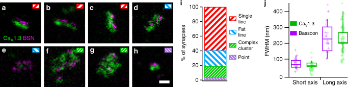
Fig. 1
2D nanoscale anatomy of IHC Ca 2+ -channel clusters. a u2013 h Representative examples of AZs assumed to run roughly perpendicular to the imaging axis at the base of IHCs, with immunofluorescence for ...
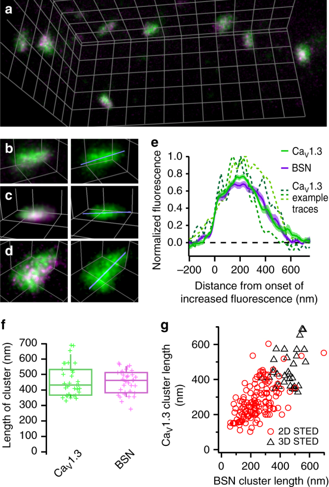
Fig. 2
3D nanoscale anatomy of IHC Ca 2+ -channel clusters. a u2013 d Volumetric displays of representative examples of Ca V 1.3 (green) and bassoon (magenta) immunofluorescence at IHC AZs, acquired with 3D-...
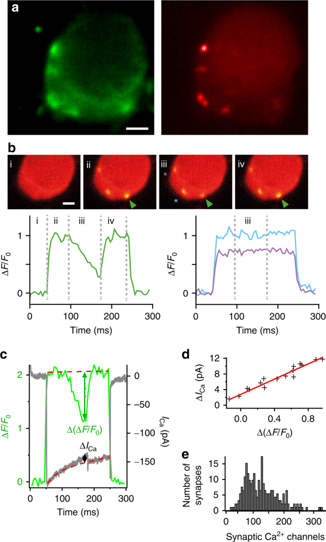
Fig. 3
Estimating the number of Ca 2+ channels per AZ by confocal Ca 2+ imaging with selective suppression of Ca 2+ influx at individual AZs. a Representative image of hotspots of depolarization-evoked Ca 2+...
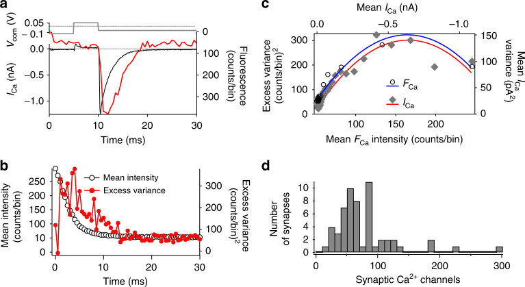
Fig. 4
Estimating the number of Ca 2+ channels per AZ by fluorescence fluctuation analysis. a Voltage protocol (upper panel) used to evoke Ca 2+ influx, visualized by the fluorescence signal ( F Ca , red tra...
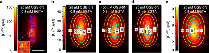
Fig. 5
Theoretical reaction/diffusion model of Ca 2+ at the IHC AZ. a Theoretical model of Ca 2+ influx at a 430u2009nmu2009u00d7u200967u2009nm cluster of 120 Ca 2+ channels (blue symbols, width of 10u2009nm...
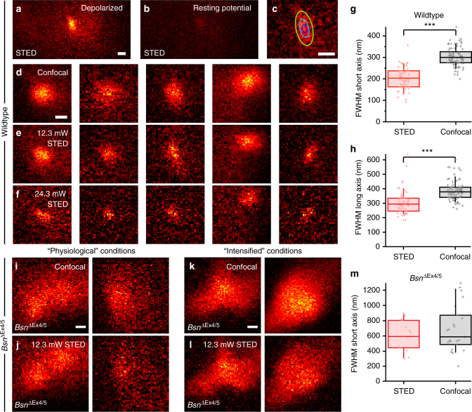
Fig. 6
Super-resolution imaging of presynaptic Ca 2+ signals in IHCs. a u2013 c Hotspot of OGB-5N fluorescence in a wildtype mouse IHC in u201cphysiological conditionsu201d (same in d u2013 f , 25u2009u00b5M...
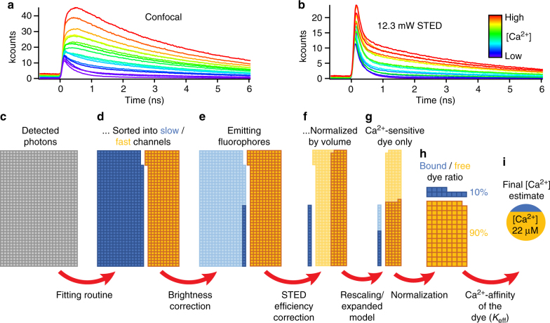
Fig. 7
Calculation of [Ca 2+ ] from measured photons by application of correction factors. a Time-correlated single photon counting (TCSPC) reveals how the fluorescence lifetime traces of OGB-5N are highly s...
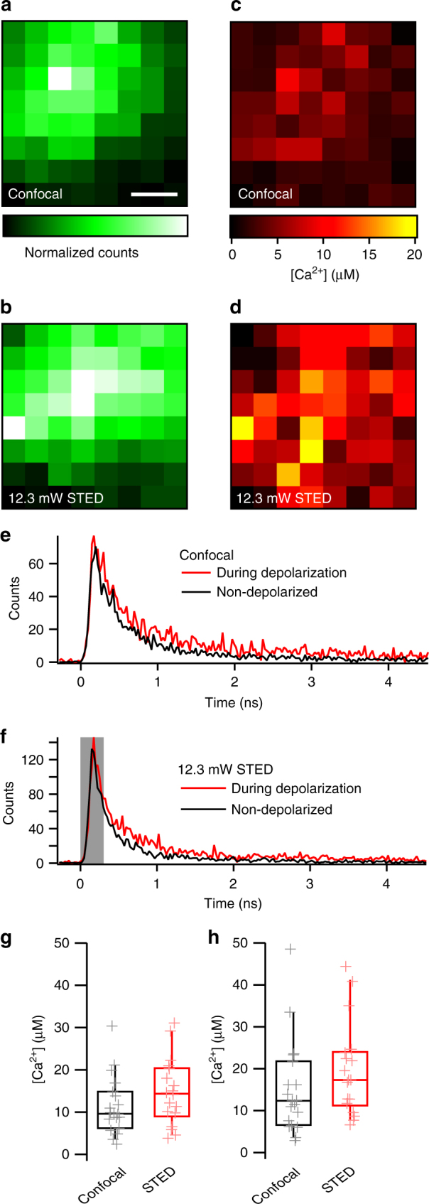
Fig. 8
Measuring synaptic Ca 2+ concentration by fluorescence lifetime imaging. a u2013 d Representative data from two 8u2009u00d7u20098 (50u2009nm steps in x and y ) pixel raster scans of a hotspot of Ca 2+...
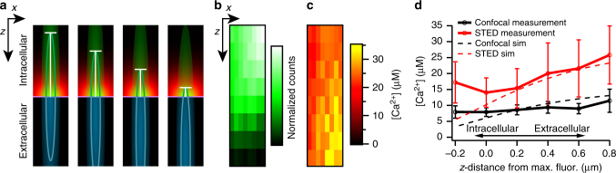
Fig. 9
Decreasing the focal volume of Ca 2+ imaging by moving the PSF in z . a Schematic drawing illustrating the decreased volume of intracellular dye that is sampled when moving the focus of the microscope...
Figure images are served from the NIH/NLM PubMed Central Open Access Subset or Europe PMC; copyright remains with the publishers and authors.
💬 Discussion
0 commentsNo comments yet. Be the first to start a discussion!
Leave a Comment