Abstract
Abstract It is essential for cells to control which genes are transcribed into RNA. In eukaryotes, two major control points are recruitment of RNA polymerase II (Pol II) into a paused state, and subsequent pause release toward transcription. Pol II recruitment and pause release occur in association with macromolecular clusters, which were proposed to be formed by a liquid–liquid phase separation mechanism. How such a phase separation mechanism relates to the interaction of Pol II with DNA during recruitment and transcription, however, remains poorly understood. Here, we use live and super‐resolution microscopy in zebrafish embryos to reveal Pol II clusters with a large variety of shapes, which can be explained by a theoretical model in which regulatory chromatin regions provide surfaces for liquid‐phase condensation at concentrations that are too low for canonical liquid–liquid phase separation. Model simulations and chemical perturbation experiments indicate that recruited Pol II contributes to the formation of these surface‐associated condensates, whereas elongating Pol II is excluded from these condensates and thereby drives their unfolding.
🔬 Techniques
🔭 Microscopes
🧬 Organisms
✨ Fluorophores
🧪 Sample Preparation
🏭 Microscope Brands
🧪 Reagent Suppliers
📷 Detectors
🔎 Objectives
💻 Software Details
💾 Data Repositories
🏛️ Research Organizations (ROR)
Affiliated research institutions:
📋 Methods
Zebrafish husbandry
Fish were raised and bred according to local regulations in the fish facility of the Institute of Biological and Chemical Systems. Embryos were obtained by spontaneous mating. Embryos were dechorionated with Pronase, washed with E3 embryo medium, and subsequently kept in agarose‐coated dishes in 0.3× Danieau's solution at 28.5°C.
Imaging of Pol II phosphorylation states in live zebrafish embryos
Covalently labelled antigen binding fragments (Fab) were injected into the yolk of dechorionated embryos at the single cell stage. Per embryo, 1 nl of Fab mix (0.2 μl 1% Phenol Red, 1.5 μl A488‐labeled anti‐Pol II Ser2P Fab, 2.3 μl Cy3‐labeled anti‐Pol II Ser5P Fab, Fab stock concentration ≈ 1 mg/ml) was injected. Embryos were mounted at the high stage in 0.7% low melting point agarose in 0.3× Danieau's solution in ibidi 35 mm imaging dishes (#1.5 selected glass cover slips). Embryos for additional fixed imaging were taken from those injected for live imaging, transferred to a fixation solution at the sphere stage (2% formaldehyde, 0.2% Tween‐20 in 0.3x Danieau's embryo media), left to fix at 4°C overnight, washed three times with Dulbecco's formulation PBS with 0.1% Tween‐20 (PBST), and mounted for imaging in VectaShield H‐1000 using #1.5 selected glass cover slips. Primary cell culture from zebrafish embryos Fish embryos were collected in the oblong stage and moved to low‐retention microcentrifuge tubes. The embryos were deyolked through vortexing in deyolking buffer (55 mM NaCl, 1.75 mMKCl, 1.25 mM NaHCO 3 ). Afterward, 1 ml PBS (Dulbecco's formulation) with 0.8 mM CaCl 2 was added to the samples and incubated for 30 min. Inhibitors were introduced to PBS before distribution to individual culturing tubes. Samples were fixed by addition of 330 μl of 8% Formaldehyde in PBS with 0.8 mM CaCl 2 to each tube. Tubes were immediately spun down at 800 g and left for 15 min at room temperature, and then, the liquid was replaced by 8% formaldehyde in PBS + CaCl 2 , left at room temperature for further fixation for at least 20 min.
Show full methods section
Zebrafish husbandry
Fish were raised and bred according to local regulations in the fish facility of the Institute of Biological and Chemical Systems. Embryos were obtained by spontaneous mating. Embryos were dechorionated with Pronase, washed with E3 embryo medium, and subsequently kept in agarose‐coated dishes in 0.3× Danieau's solution at 28.5°C.
Imaging of Pol II phosphorylation states in live zebrafish embryos
Covalently labelled antigen binding fragments (Fab) were injected into the yolk of dechorionated embryos at the single cell stage. Per embryo, 1 nl of Fab mix (0.2 μl 1% Phenol Red, 1.5 μl A488‐labeled anti‐Pol II Ser2P Fab, 2.3 μl Cy3‐labeled anti‐Pol II Ser5P Fab, Fab stock concentration ≈ 1 mg/ml) was injected. Embryos were mounted at the high stage in 0.7% low melting point agarose in 0.3× Danieau's solution in ibidi 35 mm imaging dishes (#1.5 selected glass cover slips). Embryos for additional fixed imaging were taken from those injected for live imaging, transferred to a fixation solution at the sphere stage (2% formaldehyde, 0.2% Tween‐20 in 0.3x Danieau's embryo media), left to fix at 4°C overnight, washed three times with Dulbecco's formulation PBS with 0.1% Tween‐20 (PBST), and mounted for imaging in VectaShield H‐1000 using #1.5 selected glass cover slips. Primary cell culture from zebrafish embryos Fish embryos were collected in the oblong stage and moved to low‐retention microcentrifuge tubes. The embryos were deyolked through vortexing in deyolking buffer (55 mM NaCl, 1.75 mMKCl, 1.25 mM NaHCO 3 ). Afterward, 1 ml PBS (Dulbecco's formulation) with 0.8 mM CaCl 2 was added to the samples and incubated for 30 min. Inhibitors were introduced to PBS before distribution to individual culturing tubes. Samples were fixed by addition of 330 μl of 8% Formaldehyde in PBS with 0.8 mM CaCl 2 to each tube. Tubes were immediately spun down at 800 g and left for 15 min at room temperature, and then, the liquid was replaced by 8% formaldehyde in PBS + CaCl 2 , left at room temperature for further fixation for at least 20 min.
THP‐1 cell culture
Undifferentiated cells from the human monocytic cell line THP‐1 were generously provided by the Weiss laboratory, Institute of Biological and Chemical Systems, Karlsruhe Institute of Technology (Fritsch‐Decker et al , 2018 ). Cells were transferred into low‐retention microcentrifuge tubes directly before experimental treatment, inhibitors were applied by spike‐in and incubated for 30 min at room temperature, and fixation was carried out identically to primary zebrafish cell cultures.
Inhibitor treatment
All inhibitors were resuspended in DMSO to recommended effective concentrations (Bensaude, 2011 ). Flavopiridol hydrochloride hydrate (F3055, Sigma‐Aldrich) was resuspended to a stock concentration of 12.5 mM and diluted 1:12,500 to an effective concentration of 1 μM. Actinomycin D (A1510, Sigma‐Aldrich) was resuspended to an initial concentration of 1 mg/ml and diluted 1:200 to an effective concentration of 5 μg/ml. Triptolide (T3652, Sigma‐Aldrich) was resuspended to a stock concentration of 10 mM and diluted 1:20,000 to an effective concentration of 500 nM. The effectiveness of all inhibitors was verified on the basis of Pol II phosphorylation changes at the whole nucleus level (Appendix Fig S14 ). Alpha‐amanitin (A2263, Sigma‐Aldrich) was micro‐injected into the yolk (1 nl per embryo) at a concentration of 0.2 mg/ml (dissolved in water) at the 1‐cell stage (Joseph et al , 2017 ; Hilbert et al , 2021 ). Whole embryo flavopiridol treatment was carried out by adding 10 μM flavopiridol to the embryo media (Vopalensky et al , 2018 ). Hexanediol treatment 3% w/v in PBS + 0.8 mM CaCl 2 for the last 5 min of 30‐min primary cell culture, then fixation and staining with regular immunofluorescence for instant‐SIM.
Whole embryo immunofluorescence
Whole embryo samples were obtained by fixing sphere‐stage embryos over the following night at 4°C (2% formaldehyde, 0.2% Tween‐20 in 0.3× Danieau's embryo media). Animal cap parts of these samples were permeabilized in 0.5% Triton X‐100 in PBS for 15 min at room temperature, washed three times with PBST for 10 min, and blocked in 4% BSA in PBST for at least 30 min at room temperature. Primary antibodies were applied over the following night at 4°C in 4% BSA in PBST. Secondary antibodies were applied over the following night at 4°C in 4% BSA in PBST. Primary and secondary antibodies were removed by washing three times with PBST for 5 min. After washing out the secondary antibodies, the samples were again fixed with 4% formaldehyde for 15 min for long‐term retention of antibody staining. In most cases, these post‐fixed embryo samples were free of yolk, and any remaining pieces of yolk were manually removed with fine forceps while transferring samples through three washes of PBST in glass dishes. The deyolked animal caps were mounted using selected #1.5 cover slips. The antibodies, mounting media, and DNA stains used in the different experiments are listed below.
Cell culture immunofluorescence
Fixed cell cultures were processed for the entire immunofluorescence procedure in the low‐retention microcentrifuge tubes in which they were cultured. Cells were permeabilized with 0.5% Triton X‐100 in PBS for 10 min, washed three times with PBST, and blocked with 1 ml of 4% BSA in PBST for 30 min. Primary antibodies were applied over the following night at 4°C in 4% BSA in PBST. Secondary antibodies were applied over the following night in 4% BSA in PBST. Primary and secondary antibodies were removed by washing three times with PBST. After washing out the secondary antibodies, the samples were again fixed with 8% formaldehyde in PBS for 15 min for long‐term retention of antibody staining. Samples were washed another three times with PBST and then mounted using 30 μl of VectaShield H‐1000 supplemented with a 1:2,500 dilution of Hoechst 33342 (stock concentration 20 mM) using selected #1.5 cover slips. The antibodies used in the different experiments are listed below.
STEDD sample preparation
Samples for STEDD imaging (Fig 2 ) were prepared from whole embryos. Primary antibodies (see Table 1 ): mouse anti‐Pol II Ser5P (4H8, 1:300), rabbit anti‐Pol II Ser2P ( EPR18855 , 1:2,500). Secondary antibodies (see Table 2 ): goat anti‐mouse conjugated with STAR RED (1:1,000), donkey anti‐rabbit conjugated with Alexa 488 (1:2,000). Samples were mounted in TDE‐O (Abberior). Table 1 List of primary antibodies. All primary antibodies used for immunofluorescence in this studies were monoclonal and are commercially available. Target Type Clone Supplier Cat. No. Lot No. Pol II S5P Mouse IgG 4H8 Abcam ab5408 GR205997 ‐15, GR3325973‐3 Pol II S5P Rat IgG 3E8 Active motif 61986 10618002 Pol II S2P Mouse IgM H5 Biolegend 920204 B223109 Pol II S2P Rabbit IgG EPR18855 Abcam ab193468 GR240664 ‐4, GR240664 ‐6 Pol II pan Mouse IgG 8WG16 Invitrogen MA1‐26249 VJ3115733 H3S28P Rat IgG HTA28 Abcam ab10543 GR3219690‐4 H3K27ac Rabbit IgG EP16602 Abcam ab177178 GR320298 John Wiley & Sons, Ltd Table 2 List of secondary antibodies. All secondary antibodies used for immunofluorescence in this studies were polyclonal and are commercially available. Antibody Species Fluorophore Supplier Cat. No. Anti‐mouse IgG Goat Alexa 488 Invitrogen A11001 Anti‐mouse IgG Goat Alexa 594 Invitrogen A11005 Anti‐mouse IgG Goat STAR ORANGE Abberior STORANGE‐1001‐500UG Anti‐mouse IgG Goat STAR RED Abberior 2‐0002‐011‐2 Anti‐mouse IgM Goat Alexa 594 Invitrogen A21044 Anti‐rabbit IgG Donkey Alexa 488 Invitrogen A21206 Anti‐rabbit IgG Goat Alexa 594 Invitrogen A11037 Anti‐rabbit IgG Goat STAR 520 SXP Abberior ST520SXP‐1002‐500UG Anti‐rabbit IgG Goat STAR ORANGE Abberior STORANGE‐1002‐500UG Anti‐rat IgG Goat Alexa 594 Invitrogen A11007 Anti‐rat IgG Goat Alexa 647 Invitrogen A21247 John Wiley & Sons, Ltd Two‐color STED sample preparation Samples for two‐color STED imaging (Appendix Fig S6 ) were prepared from whole embryos. Two sets of primary and secondary antibodies were used (see Table 1 and Table 2 ). The first set of antibodies (AB set 1) contained as primary antibodies: mouse IgG anti‐Pol II Ser5P (4H8, 1:300), rabbit IgG anti‐Pol II Ser2P ( EPR18855 , 1:300). Secondary antibodies: goat anti‐mouse conjugated with STAR RED (1:300), goat anti‐rabbit conjugated with STAR ORANGE (1:300). The second set of antibodies (AB set 2) contained as primary antibodies: rat IgG anti‐Pol II Ser5P (3E8, 1:300), mouse IgM anti‐Pol II Ser2P (H5, 1:300). Secondary antibodies: goat anti‐rat conjugated with Alexa 647 (1:300), goat anti‐mouse IgG conjugated with Alexa 594 (1:300). Samples were mounted in TDE‐O (Abberior).
Sample preparation from hexanediol and inhibitor treated cell cultures
Samples were obtained from cell cultures treated with hexanediol (Fig 3 ) or different transcription inhibitors (Appendix Figs S10, S14 and S15 ). Primary antibodies (see Table 1 ): mouse anti‐Pol II Ser5P (4H8, 1:1,000), rabbit anti‐Pol II Ser2P ( EPR18855 , 1:1,000), rat anti‐H3S28P (HTA28, 1:10,000). Secondary antibodies (see Table 2 ): goat anti‐mouse conjugated with Alexa 488 (1:1,000), goat anti‐rabbit conjugated with Alexa 594 (1:1,000), goat anti‐rat conjugated with Alexa 647 (1:1,000).
Three‐color STED sample preparation
Samples for three‐color STED imaging (Fig 3D and E ) were prepared from whole embryos. Primary antibodies (see Table 1 ): mouse anti‐Pol II Ser5P (4H8, 1:300), rabbit anti‐H3K27ac (EP16602, 1:300). Secondary antibodies (see Table 2 ): goat anti‐mouse conjugated with Alexa 594 (1:300), goat anti‐rabbit conjugated with STAR 520 SXP (1:300). Samples were mounted in glycerol with 10 μM JF646‐Hoechst (gift from the Lavis Lab) (Legant et al , 2016 ; Spahn et al , 2019 ; Zhang et al , 2019 ).
Oligopaint FISH sample preparation
Samples for combined oligopaint DNA FISH and immunofluorescence (Fig 4F and G ) were prepared from whole embryos. Primary antibodies (see Table 1 ): mouse anti‐Pol II Ser5P (4H8, 1:300), rabbit anti‐Pol II Ser2P ( EPR18855 , 1:300). Secondary antibodies (see Table 2 ): goat anti‐mouse conjugated with STAR RED (1:300), goat anti‐rabbit conjugated with Alexa 488 (1:300). Sample preparation for not phospho‐specific visualization of Pol II Samples for the assessment of general Pol II levels after triptolide and alpha‐amanitin treatment (Appendix Fig S16A and B ) were prepared from primary zebrafish cell cultures. Primary antibodies (see Table 1 ): mouse anti‐Pol II (pan CTD, 8WG16, 1:1,000). Secondary antibodies (see Table 2 ): goat anti‐mouse conjugated with Alexa 594 (1:1,000). ChIP‐seq analysis Raw ChIP‐seq reads were obtained for Pol II Ser5P at dome ( GSE4426 (Zhang et al , 2014 )), H3K27ac at dome ( GSE32483 (Bogdanović et al , 2012 )), input at dome ( GSE84602 (Meier et al , 2018 )), H3K27ac at 80% epiboly ( GSE32483 (Bogdanović et al , 2012 )), and input at 80% epiboly ( GSE41458 (Winata et al , 2013 )). Raw reads were aligned to the zebrafish genome (danRer10) using Bowtie 2 (Langmead et al , 2009 ), filtering out reads with more than 1 mismatch using samtools (Li et al , 2009 ). For coverage tracks, bigWig files were generated and tracks were produced using pyGenomeTracks (Lopez‐Delisle et al , 2021 ). Pol II Ser5P and H3K27ac peaks were called using macs2 callpeak from MACS2 (Zhang et al , 2008 ), with Input as control and reads extended to the predicted fragment length from macs2 predictd .
Identification of super‐enhancers followed previous work in zebrafish
(Pérez‐Rico et al , 2017 ), using the program ROSE (Lovén et al , 2013 ; Whyte et al , 2013 ) on the H3K27ac peaks. This removes peaks within 2.5 kb of a transcription start site, stitches together the remaining peaks if they are closer than 12.5 kbs, and identifies super‐enhancers from the resulting list after ranking them by their H3K27ac signal. All underlying pipelines and scripts are provided as a Zenodo repository, see Data availability . Oligopaint DNA FISH Genome homology region oligos for the entire zebrafish genome were used as provided by OligoMiner (Beliveau et al , 2018 ). Six loci with a strong Pol II Ser5P signal in the super‐enhancer window were selected from the list of identified super‐enhancers at the dome stage (SE1–SE6). Two sets of controls were selected: three super‐enhancer loci without a strong Pol II Ser5P signal (SE7–SE9), and three super‐enhancer loci from 80% epiboly, which are not identified as super‐enhancers at the dome stage (SE10–SE12). Additionally, four gene loci with strong H3K27ac signal and strong Ser5P signal in the promoter ( crsp7 , celf1 ) or gene body ( cdc25b , rnf19a ) were selected. Around each of these 16 loci, regions ranging between 25 and 100 kb were chosen, so as to obtain at least 300 homology oligos per region. In total, for the 16 regions, 5,989 oligopaint homology oligos were obtained. Primers were designed with the OligoLego tool (Nir et al , 2018 ), and joined to the homology oligos and streets (to which primers bind) to construct oligopaint probes that formed the oligopaint library. The primers were first validated to be potential PCR primers, filtered out to ensure that they do not adopt secondary structures, screened in pairs to avoid cross‐talk when hybridizing, and finally aligned against the zebrafish genome to ensure that none of them align with the genome. A penalty matrix was then built to determine compatibility of possible street pairs. The final oligopaint library was then compiled by appending the streets and the hybridizing oligos in the required configuration, consisting of a universal mainstreet (to which the universal forward primer binds), a locus‐specific mainstreet (to which a locus‐specific forward primer binds), a different universal mainstreet (to which a fluorescent forward primer binds), the homology region oligo (that hybridizes to the target loci), and a universal backstreet (to which the universal reverse primer binds). The oligopaint library was synthesized by Twist Biosciences. All underlying pipelines, scripts, and oligo tables are provided as a Zenodo repository, see Data availability . PCR amplification of oligopaint library The synthesized oligopaint library was resuspended in 10 mM Tris buffer (pH 8.0) to a final concentration of 20 ng/μl. The oligopaint library amplification was performed by PCR, using following reagents: 1 μl 10 μM universal forward primer, 1 μl 10 μM reverse primer, 1 μl dNTPs (New England BioLabs, N0447S), 0.5 μl Q5 High‐Fidelity DNA Polymerase (New England BioLabs, M0491S), 5 μl Q5 Buffer, 5 μl GC enhancer, 11 μl ddH 2 O, and 0.5 μl oligopaint library. The PCR cycles were as follows: incubation at 98°C for 3 min, followed by twelve cycles of 20 s at 98°C, 15 s at 53°C, and 15 s 72°C, with a final elongation for 1 min at 72°C. Cleaning after oligopaint library amplification The amplified oligopaint library was cleaned using DNA Clean & Concentrator‐5 kit (Zymo Research, DCC‐5). 25‐μl PCR product was mixed with 175 μl Zymo DNA binding buffer, transferred to a Zymo DCC‐5 column, and spun at 16,000 g for 1 min. Next, 200 μl DNA wash buffer was added to the column and centrifuged at 16,000 g for 1 min. The wash step was repeated. The flow‐through was discarded, and the column was spun at 16,000 g for 1 min once more. The column was transferred to a clean 1.5‐ml tube, and 30 μl ddH 2 O was added. The column was incubated at room temperature for 1 min and centrifuged at 16,000 g for 1 min. The concentration was measured using a NanoDrop device.
PCR amplification of oligopaint probes
For probe amplification, a working concentration of 2 ng/μl of the oligopaint library was prepared. The oligopaint probes were amplified using PCR. The amplification mix was prepared as follows: 2.5 μl 10 μM gene‐specific forward primer, 2.5 μl 10 μM reverse primer with T7 promoter sequence (T7 promoter sequence: TAATACGACTCACTATAGGG), 2.5 μl dNTPs, 0.5 μl Q5 High‐Fidelity DNA Polymerase, 10 μl Q5 Buffer, 10 μl GC enhancer, 19.5 μl ddH 2 O, and 2.5 μl oligopaint library. The PCR cycles were as follows: incubation for 5 min at 98°C, followed by 43 cycles of incubation at 98°C for 30 s, 58°C for 30 s, and 72°C for 15 s, with a final elongation for 5 min at 72°C. Cleaning after oligopaint probe amplification The oligopaint probes were cleaned using the DNA Clean & Concentrator‐5 kit (Zymo Research, DCC‐5). 50 μl PCR product was mixed with 350 μl Zymo DNA binding buffer, transferred to a Zymo DCC‐5 column, and spun at 16,000 g for 1 min. Afterward, 200 μl DNA Wash Buffer was added to the column and centrifuged at 16,000 g for 1 min. The wash step was repeated. The flow‐through was discarded, and the column was spun at 16,000 g for 1 min. The column was transferred to a clean 1.5‐ml tube, and 11 μl ddH 2 O was added. The samples were incubated at room temperature for 1 min and centrifuged at 16,000 g for 1 min. T7 Reaction— in vitro transcription and fluorophore attachment The amplified probe set was in vitro transcribed using a HiScribe T7 Quick High Yield RNA Synthesis Kit (New England BioLabs, E2050S). Each probe set was prepared as follows: 10 μl PCR product, 10 μl NTP buffer mix (from HiScribe kit), 2 μl T7 Polymerase mix (from HiScribe kit), 0.5 μl Recombinant RNasin (Promega, N2511), and 7.5 μl ddH 2 O. The samples were incubated at 37°C in the PCR machine for 4 h. For reverse transcription and fluorophore attachment, M‐MuLV Reverse Transcriptase (New England BioLabs, M0253L) was used. Each probe was prepared as follows: 7 μl dNTPs (New England BioLabs, N0447S), 7 μl 10× M‐MuLV Buffer, 10 μl of 100 μM A594‐labeled forward primer, 1.2 μl M‐MuLV enzyme, 1.4 μl recombinant RNasin, 13.4 μl nuclease‐free water, and 30 μl RNA from the T7 reaction. The reaction mix was incubated at 50°C for 2 h.
Cleaning of the oligopaint probes
To obtain ready‐to‐use oligopaint probes, the reverse transcription products were cleaned up using DNA Clean & Concentrator‐25 kit (Zymo Research, DCC‐25). 140 μl Oligo binding buffer (Zymo Research, D4060‐1‐40) was added to the reverse transcription reaction product, and the sample was mixed. To each sample, 560 μl of 96% ethanol was added and the sample was mixed. The solution was transferred into a Zymo DCC‐25 column and spun at 16,000 g for 1 min. The flow‐through was discarded. Afterward, 750 μl DNA Wash Buffer was added on the column and spun at 16,000 g for 1 min. The wash step was repeated. The flow‐through was discarded, and the column was transferred to a clean 1.5‐ml tube. DNA was eluted in 30 μl ddH 2 O, and the concentration was measured using a NanoDrop device. The concentration of all purified probes was higher than 3,900 ng/μl.
Sample permeabilization
Animal caps of fixed embryos were permeabilized in 0.5% Triton X‐100 in PBS for 15 min. The animal caps were washed once with 1 ml PBST for 2 min and subsequently treated with 0.1 M HCl for 5 min. The samples were washed twice with 1 ml 2× saline sodium citrate buffer with 1% Tween‐20 (2 × SSCT). Subsequently, the samples were washed with 2 × SSCT + 50% formamide solution for 2 min in room temperature, and once with 2xSSCT+50% formamide at 60°C for 20 min.
Sample denaturation and hybridization
Liquid was removed and hybridization mix was added, consisting of: 50 μl formamide, 25 μl 4× hybridization buffer (40% dextran sulfate, 8 × SSC, 0.8% Tween‐20), 4 μl 10 μg/μl RNase A, 10 μM oligopaint probes labeled with Alexa 594, and ddH 2 O added to reach a total volume of 100 μl. Samples were denatured at 90°C for 3 min and hybridized over the following night at 37°C. Post‐hybridization washes The samples were washed four times with 2 × SSCT at 60°C for 5 min. 2 × SSCT was added and incubated for 5 min at room temperature twice. Before proceeding with the immunofluorescence protocol, the samples were washed three times for 5 min in PBST. These procedures were followed by the steps described in the immunofluorescence section. Instantaneous structured illumination microscopy (instant‐SIM) Microscopy data from live whole embryos and inhibitor‐treated, fixed cells were recorded using a VisiTech iSIM high‐speed super‐resolution confocal microscope based on the instant‐SIM principle (York et al , 2013 ). The microscope was built on a Nikon Ti2‐E stand. A Nikon Silicone Immersion Objective (NA 1.35, CFI SR HP Plan Apochromat Lambda S 100XC Sil) was used for live imaging, and a Nikon Oil Immersion Objective (NA 1.49, CFI SR HP Apo TIRF 100XAC Oil) was used for fixed cell imaging. Excitation lasers at 405, 488, 561, and 640 nm were used, and illumination and acquisition settings were kept constant across all samples of a given experimental repeat. Color channels were recorded on two cameras simultaneously for increased speed during live imaging, and sequentially to avoid cross‐talk during fixed cell imaging.
Stimulated emission double depletion microscopy
Microscopy data from animal caps of fixed whole embryos were recorded using a custom‐built STEDD microscope, as previously described (Zhang et al , 2019 ). The STEDD principle allows suppression of low‐frequency image components as well as out‐of‐focus light and aberrant signal from reexcitation effects (Gao & Nienhaus, 2017 ; Gao et al , 2017 ). Here, STEDD‐resolved images were recorded using excitation by a 640 nm pulsed laser (675/55 nm (center/width) detection band‐pass filter), depletion by a titanium‐sapphire depletion laser tuned to 779 nm, and focused through an oil‐immersion objective (HCX PL APO CS 100×/1.46, Leica). The confocal image was acquired in an additional scan in the same focal plane, using a 473 nm excitation laser (520/50 nm (center/width) detection band‐pass filter) without additional depletion. Two‐ and three‐color stimulated emission depletion microscopy Data from animal caps were recorded with a Leica TCS SP8 STED microscope with a 775‐nm depletion line and a white light laser with adjustable emission wavelengths, using a motorized‐correction 93× NA 1.30 glycerol objective (HC PL APO 93×/1.30 GLYC motCORR), two HyD detectors for two‐color detection, and an additional photomultiplier tube (PMT) detector for three‐color detection. Two‐color detection based on the fluorophores STAR RED and STAR ORANGE used the following settings: color channel 1—excitation wavelength 638 nm, detection window 648–750 nm, detector gating 0.9–12 ns; color channel 2—excitation wavelength 590 nm, HyD detector window 600–630 nm, detector gating 0.3–9 ns. The STED depletion was set to 100% 3D‐STED. Two‐color detection based on the fluorophores Alexa 594 and Alexa 647 used the following settings: color channel 1—excitation wavelength 594 nm, HyD detector window 604–640 nm, detector gating 0.7–12 ns; color channel 2—excitation wavelength 640 nm, HyD detector window 650–720 nm, detector gating 0.3–9 ns. The STED depletion was set to 25% 3D‐STED. Three‐color detection was based on the DNA stain JF646‐Hoechst, the fluorophore Alexa 594, and the large Stokes shift fluorophore STAR 520 SXP, using the following settings: channel 1—excitation wavelength 640 nm, HyD detector window 661–741 nm, time gating window 1.5–9 ns; channel 2—excitation wavelength 590 nm, HyD detector window 600–660 nm, time gating window 1–9 ns; channel 3—excitation wavelength 514 nm, PMT detector window 540–600 nm, ungated detection. The STED depletion power was set to 25% 3D‐STED.
Image analysis—general overview
Image analysis was carried out using FIJI (Schindelin et al , 2012 ) and CellProfiler (McQuin et al , 2018 ) combined with Python for data handling, as well as MatLab combined with the Open Microscopy Environment BioFormats importer functionality provided by bfmatlab (Goldberg et al , 2005 ). The following provides an overview of the key image analysis steps carried out for all figures included in this study. The underlying raw image data and all pipelines and scripts are provided as Zenodo repositories indicated in each section.
Image analysis—relationship of Pol
II phosphorylation and cluster morphology in STEDD microscopy data
These analyses (Fig 2 ) were carried out in MatLab. The raw data and analysis scripts are available via Zenodo, see Data availability . Nuclear segmentation masks were obtained by Gaussian blur ( σ = 1.2 μm) and Otsu thresholding of the Pol II Ser5P channel. Pol II Ser5P clusters and Pol II Ser2P spots were segmented by local background subtraction (Gaussian blur image with σ = 0.4 μm subtracted), followed by global robust background thresholding (0.5 and 0.25 Standard Deviations), respectively. For each Pol II Ser5P cluster, mean intensity, area, and solidity were extracted. For Pol II Ser2P spots, only the mean intensity was extracted due to the lower confocal resolution relative to the STEDD data.
Image analysis—changes in Pol II
Ser2P upon flavopiridol treatment of whole embryos These analyses (Appendix Fig S5 ) were carried out in MatLab. The raw data and analysis scripts are available via Zenodo, see Data availability . Nuclei were segmented by Otsu thresholding of the blurred (Gaussian kernel with σ = 0.3 μm) and background‐subtracted (Gaussian kernel with σ = 5 μm) Pol II Ser5P channel. Cytoplasmic background was subtracted using secondary masks, which were obtained by dilation to 1.0 and 1.5 μm of the primary nuclear masks.
Image analysis—Pol II phosphorylation and cluster morphology in instant‐SIM data
These analyses (Appendix Figs S3, S14 and S15 ) were carried out in CellProfiler. The raw data and analysis pipeline and scripts are available via Zenodo, see Data availability . Z‐stacks were maximum‐intensity‐projected in FIJI, including a range of 25 slices visually chosen for best image quality from a given z‐stack. The further 2D analysis was implemented as a CellProfiler pipeline. Specifically, a two‐step approach was used, where first cell nuclei and subsequently Pol II clusters inside nuclei were segmented based on the Pol II Ser5P signal. Nuclei segmentation masks were obtained by global Otsu thresholding. Cytoplasmic masks were generated by outward dilation (25 pixels) from the nuclear masks. Pol II clusters inside nuclei were obtained by enhancing the Pol II Ser5P channel (speckle enhancement) and global robust background thresholding (5.5 standard deviations). For each cluster, the mean Pol II Ser5P and Pol II Ser2P intensities (cytoplasmic background subtracted on per‐nucleus basis), cluster area, and cluster solidity were extracted. The mean intensity of Pol II Ser5P and Pol II Ser2P in the nuclei, cytoplasm, and in single clusters was measured. The geometric properties—solidity, area—were measured for each cluster. All clusters smaller than four pixels were discarded. Further data processing and graph preparation were done in Python. Data from fixed cells were analyzed in the same way, except that, as a first step, the additional color channels with DNA and Histone 3 serine 28 phosphorylation (H3Ser28P, used to detect cells in prophase) signal were used to establish Otsu‐threshold masks for nuclear segmentation and prophase exclusion, respectively. In the robust background segmentation of Pol II Ser5P clusters, 6.5 standard deviations were chosen for zebrafish primary cell cultures, 8 standard deviations for THP‐1 cell cultures. A comparison of our analysis based on two‐dimensional, maximum‐intensity‐projected images with an analysis of full three‐dimensional stacks showed a good correlation between both approaches (Appendix Fig S2A and B ). Image analysis—analysis of Pol II Ser5P / Ser2P colocalization in two‐color STED data These analyses (Appendix Fig S6 ) were carried out in MatLab. The raw data and analysis pipeline and scripts are available via Zenodo, see Data availability . Images were two‐dimensional and contained one nucleus per image. The nucleus was segmented by Otsu thresholding of the blurred Pol II Ser5P channel ( σ = 1.2 μm). Pol II Ser5P and Pol II Ser2P foci were segmented by application of a robust background threshold within the segmented nucleus (2.0 and 3.0 standard deviations, respectively). The Pol II Ser5P channel was background‐subtracted prior to segmentation (Gaussian blur with σ = 0.3 μm). Mean intensities of clusters were calculated using Ser5P segmentation masks and normalized against whole nucleus median intensity on a per‐nucleus level. Overlap was quantified by use of the Pol II Ser5P and Pol II Ser2P segmentation masks, and quantified in terms of percentage of all Pol II Ser2P mask pixels in a given nucleus.
Image analysis—Pol II Ser5P clusters and Pol II
Ser2P spots after hexanediol treatment
These analyses (Fig 3 ) were carried out in MatLab. The raw data and analysis pipeline and scripts are available via Zenodo, see Data availability . Z‐stacks were maximum‐intensity‐projected in FIJI, including a range of 25 slices visually chosen for best image quality from a given z stack. The further analysis was carried out in MatLab. Nuclei in a given z projection were segmented by Otsu thresholding of the blurred Pol II Ser5P channel ( σ = 1.2 μm). Pol II Ser5P clusters and Pol II Ser2P foci were segmented by application of a robust background threshold within the segmented nucleus (4 and 4 standard deviations, respectively). Both channels were background‐subtracted prior to segmentation (Gaussian blur with σ = 0.5 μm). Area and solidity of a given object were calculated from Pol II Ser5P and Pol II Ser2P segmentation masks.
Image analysis—H3K27ac and DNA distribution with respect to Pol II
Ser5P clusters These analyses (Fig 4D and E ) were carried out in MatLab. The raw data and analysis pipeline and scripts are available via Zenodo, see Data availability . STED reexcitation signal in the DNA channel was reduced by subtracting a Gaussian‐blurred ( σ = 0.1 μm) image recorded with only the STED laser activated. Images were two‐dimensional and contained one nucleus per image. The nucleus was segmented by Otsu thresholding of the blurred DNA channel ( σ = 1.2 μm). Pol II Ser5P foci were segmented by application of a robust background threshold within the segmented nucleus (2.5 standard deviations). The Pol II Ser5P channel was background‐subtracted prior to segmentation (Gaussian blur with σ = 2 μm). Mean intensities were calculated from Pol II Ser5P segmentation masks and normalized against whole nucleus median intensity on a per‐nucleus level.
Image analysis—oligopaint signals in relation to Ser5P clusters
These analyses (Fig 4F and G ) were carried out in MatLab. The raw data and analysis pipeline and scripts are available via Zenodo, see Data availability . All analysis operations were carried out under consideration of three‐dimensional organization. Each image stack typically contained several nuclei, which were segmented by Otsu thresholding of the blurred (Gaussian kernel with σ = 1 μm) and background‐subtracted (Gaussian kernel with σ = 10 μm) Pol II Ser5P channel. Pol II Ser5P clusters and oligopaint‐labeled regions were segmented by application of a robust background threshold within the segmented nuclei (2 and 6 standard deviations, respectively). The Pol II Ser5P channel was background‐subtracted (Gaussian kernel with σ = 3 μm) prior to segmentation. The oligopaint channel was background‐subtracted (Gaussian kernel with σ = 5 μm) and smoothed (Gaussian kernel with σ = 0.1 μm) prior to segmentation. Mean intensities were calculated from oligopaint segmentation masks and normalized against whole nucleus median intensity on a per‐nucleus level. The distance between oligopaint‐labeled regions and Pol II Ser5P clusters was assessed for each oligopaint‐labeled region, using the Euclidean distance to the nearest Pol II Ser5P cluster. Euclidean distance was calculated between centroids of segmentation masks.
Statistics
Box plots conform to standard practice (median, quartiles as boxes, range as whiskers, outliers removed outside of 1.5 times interquartile range extension). Statistical significance was indicated for differences of mean or median (as indicated) relative to the control or comparison condition, two‐tailed permutation test; *, **, and *** indicate P < 0.05, P < 0.01, and P < 0.001, respectively; and n.s. indicates no statistically significant difference ( P ≥ 0.05). Significance levels were Bonferroni‐corrected for multiple comparisons (division by number of comparisons), leading to lowered significance levels as indicated. The permutation test is based on a computational resampling procedure, which we sampled to an accuracy of P = 0.0001, lower values are stated as P < 0.0001.
Lattice model
Lattice kinetic Monte Carlo model
We describe the Pol II cluster morphologies observed in zebrafish experiments using a simple physical model, which is limited to the most essential components: particles corresponding to a Pol II Ser5P‐rich component (in the following abbreviated as Pol II particles) and linear polymer chains with different subregions corresponding to chromatin. To obtain spatial configurations of this system, we used a rejection‐free lattice kinetic Monte Carlo (LKMC) algorithm. LKMC algorithms, generally speaking, are suited to simulate coarse‐grained stochastic non‐equilibrium systems. The rejection‐free algorithm (Appendix Fig S9A ) is similar to the Gillespie algorithm (Gillespie, 1977 ). At the beginning of a simulation, by checking the system configuration and nearest neighbors of every particle within the system, a rate catalog with all possible transitions is created, providing also the total system rate as the sum of all transition rates. This initial cataloging step is followed by a Monte Carlo (MC) routine that is repeated N times. During each step, one of the previously defined transitions is randomly selected while associating transitions with a higher rate with a higher likelihood of occurrence. The transition is then performed and changes the system state. This is followed by a local update of the possible transitions in the affected lattice area, the total rate of the system, and the system time. This simulation paradigm has been used to model surface catalysis processes (Hoffmann et al , 2014 ) and slip‐link DNA systems with DNA polymers and ring proteins (Miermans & Broedersz, 2020 ). The initialization of the simulations proceeds similar to the latter work, but instead of ring proteins uses the Pol II particles in addition to the polymers. Initial configuration Chromatin is modeled as a connected polymer chain with different internal states: inactive (black), regulatory (blue), and active (gray). Exclusion from occupied volume is assumed, so that chains can only undergo a limited type of moves that maintain chain connectivity. Pol II particles (single lattice sites, red) can freely diffuse in space and interact with different affinities w i with the chromatin polymer and other Pol II particles. The different interspecies affinities of Pol II particles to specific subregions of a chain allow us to study the formation of Pol II clusters in the framework of microphase separation. At the beginning of a given simulation, the Pol II particles are randomly distributed on the 25 × 25 lattice. The chromatin polymer was placed in different initial configurations (e.g., single chain, cross of four chains, four parallel chains, four chains organized as random walks). The monomers making up chromatin chains were assigned to the different colors, giving contiguous sections of black polymer (number of monomers: N IC ), blue monomers ( N RC ), and gray monomers ( N AC ). The number of red particles ( N S5P ) can be varied. Pol II particle and polymer move set After initialization and each time step, the rate catalog is updated. To find all possible transitions of the system for the rate catalog, we first have to define the allowed move set for every species. The Pol II particles are allowed to move to one of its eight nearest neighbors in one MC step (Appendix Fig S9D , left). The polymer is simulated as a connected and self‐avoiding chain. We therefore use the common Verdier‐Stockmayer move set, consisting of end‐bond flip, kink‐jump, and a crankshaft move (Appendix Fig S9D , right) (Verdier & Stockmayer, 1962 ; Hilhorst & Deutch, 1975 ; Miermans & Broedersz, 2020 ). Movements to positions outside the lattice are not considered. The end‐bond flip can occur only for the first or last monomer of the polymer and moves the first/last monomer to any lattice site neighboring the second/second‐last particle of the polymer, changing the angle between the old and new positions by 90 degrees. For a kink jump, a monomer is moved to the opposite side of a corner formed by the preceding monomer, the monomer itself, and the subsequent monomer. To reach ergodicity of the system, a third move, called the crankshaft move, is added (Hilhorst & Deutch, 1975 ). While the end‐bond flip and the kink jump move only one monomer, the crankshaft move changes the position of two successive monomers. Rate catalog To draw up the rate catalog, we first browse all Pol II‐particle positions within the lattice and test the occupation of its eight nearest neighbors. Those that are not occupied by the same species are possible directions for transitions within the system. Together with the defined rate coefficient, k p = 0.1, and the Arrhenius equation, k = k p · e ‐ ( E 2 ‐ E 1 ) , the rate for each transition can be determined. The energies before ( E 1 ) and after ( E 2 ) are stated in units of k B T , where T is the system's temperature, and are determined under consideration of the different interspecies affinities between the swapped particles and their nearest neighbors (Appendix Fig S9C ). Where a nearest neighbor position is located outside the lattice, no energy contribution is added for that neighbor. For every Pol II‐particle transition, the old and new position and also the rate for the transition are added to the rate catalog. The transition rate is also added to the overall system rate k total . As a second step, the same procedure is carried out for moves of the polymer chain. Initially, the position within the polymer and also the position of the previous and subsequent monomers are checked. Depending on the position and configuration, only certain movements of the monomer are possible. As with the Pol II particles, it must then be checked whether the possible new position resulting from the move is already occupied by another monomer. If this is not the case, the Arrhenius equation and the rate coefficient for a single move (same as k kink ) are used to determine the rate of the transition. Since the crankshaft move affects two monomers at the same time, this coefficient is smaller compared to the other moves, k crank = k kink ⋅log 4/3 (Miermans & Broedersz, 2020 ). The polymer transitions are also added to the rate catalog. In addition to the positions and rates, the specific type of movement is added. Furthermore, for the crankshaft move both positions before and after the respective move are saved. Now all required properties of the system are defined and the main part of the Monte Carlo simulation can start. Perform move (MC‐Step) In this section, the core iteration step of the algorithm is described. At first, we draw a transition out of the previously defined rate catalog. This is done using a uniformly distributed random number r 1 from the interval (0,1], the total rate k total , and the tower‐sampling method (Appendix Fig S9E ). The transition is chosen using the quantity k * = r 1 ⋅ k total . In particular, by looping through all transitions within the catalog and summing up each individual rate k i , we identify a transition j with rate k j such that the relation ∑ i j ‐ 1 k i < k ∗ ≤ ∑ i j k i is fulfilled. The chosen transition is then performed and the system lattice is updated. The system time is also updated by adding Δ t = ‐ log ( r 2 ) k total with a second random number r 2 from (0,1] to the current system time t (Miermans & Broedersz, 2020 ). This routine is performed N times. Local update At the end of each of the above iteration steps, the system rate catalog has to be updated. In the simplest approach, we delete the previous rate catalog and completely recalculate it. While formally correct, more computationally efficient alternative approaches are available (Miermans & Broedersz, 2020 ). Position changes in the simulation are only made in a confined area surrounding the particle that is moved. Accordingly, only the transitions falling within this area need to be updated. We therefore determine all transitions leading to a position within this area, or whose origin is within this area and update only these transitions. Since the longest transition within the system is performed by the crankshaft move with a distance of two lattice sites, the local update has to be performed in the region [ x ± 4, y ± 4] (Appendix Fig S9F ). Parameter adjustment Besides the self‐affinity of Pol II particles, w S5P‐S5P (interaction energy measured in units of k B T ; Fig 5 ), we also adjusted the number of Pol II particles, N S5P , and Pol II‐particle affinity to regulatory chromatin, w RC‐S5P . To adjust N S5P , we add a single polymer chain of length L Polymer = 20 with black and blue subregions to the simulation (Appendix Fig S10A ). We use the previously determined affinity w S5P‐S5P = −0.35, and assign w RC‐S5P = −0.5 as a preliminary value. We then varied the number of Pol II particles ( N S5P = 10, 25, 50, 100, 200). Since we planned to perform simulations with four or more polymers and different lengths of the blue regions, we choose N S5P = 100 so as to provide enough material for cluster formation (Appendix Fig S10A ). To assess the preliminary w RC‐S5P = −0.5 value, we performed simulations containing a single polymer chain ( L Polymer = 8) that consists only of blue subregions, using again w S5P‐S5P = −0.35 and the previously determined amount of Pol II particles. As we vary w RC‐S5P = −0.1, −0.3, −0.5, −0.7, −1.0, we find that the only parameter for which not the whole polymer is covered by Pol II particles (blue still visible) is w RC‐S5P = −0.1 (Appendix Fig S10B ). For all tested values, cluster formation occurs, so that we continued using the preliminary value w S5P‐S5P = −0.5, which falls in the middle region of the tested interval. Although a main aim of our model was to describe the physical mechanism of cluster formation, and not to reproduce experimental data in absolute numbers, we briefly comment on how biologically realistic the assigned parameter values are. The affinities, which determine much of the model behavior, are closely comparable to those used in our previous work (Hilbert et al , 2021 ), where we describe the organization of euchromatin as a result of RNA polymerase II transcriptional activity. Also similar to this work, we can approximately set the distance between two lattice sites equivalent to the edge length of a pixel in our instant‐SIM microscopy images (≈ 65 nm). The area of large simulated clusters (≈ 100 lattice sites, see Fig 6B ) thus corresponds to ≈ 0.43 μm 2 , which agrees very well with areas of large clusters seen in our experiments (Fig 2C ). Further, by assigning regulatory and active regions of similar length to the chromatin chains, the relative lengths seen in our ChIP‐seq analysis are reproduced (Fig 4A and B ).
Image processing
Synthetic microscopy images were obtained by converting lattice distributions of red monomers, gray polymer regions, and blue polymer regions into matrices with values 0 (unoccupied) or 1 (occupied), which were blurred with a Gaussian kernel ( σ = 1, in units of pixels). For these synthetic color channels, artificial detector noise was added in the form of Poisson‐distributed random numbers (mean λ = 5, divided by 100 before addition). Objects corresponding to Pol II Ser5P clusters were obtained from the blurred distributions of red particles using a segmentation threshold of 0.35 followed by connected‐component analysis (8‐connectivity, components with less than 10 pixels were excluded). Distributions of area, solidity, and intensity of these objects were obtained by sampling simulations at different time points (ergodic sampling). The numerical simulation and the analysis of synthetic images were carried out using Python.
Supporting information Appendix Click here for additional data file.
📊 Figures
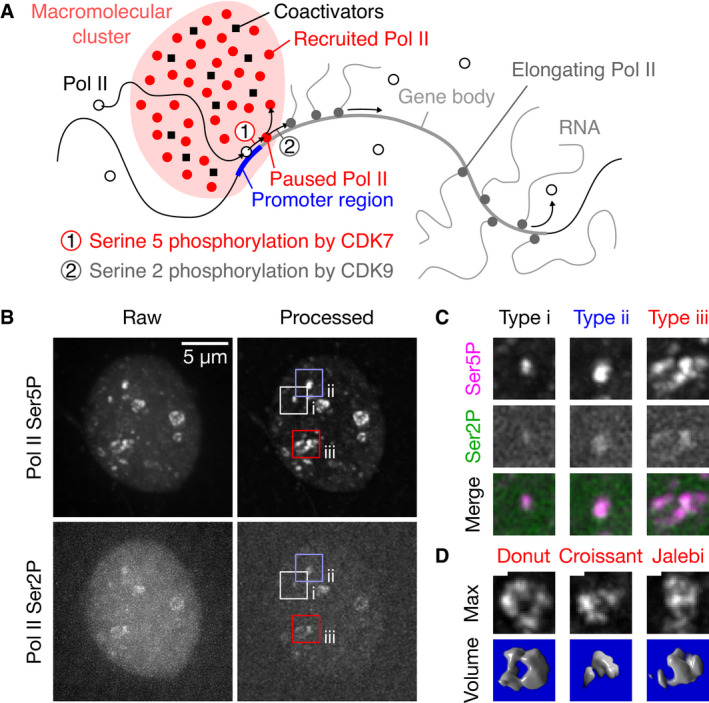
Figure 1
Phosphorylationu2010specific detection of RNA polymerase II reveals clusters displaying a variety of morphologies
Sketch of the recruitment and pause release of RNA polymerase II (Pol II) in the context of macromolecular clusters. Representative maximumu2010intensity projection of a nucleus in a live zebrafish em...
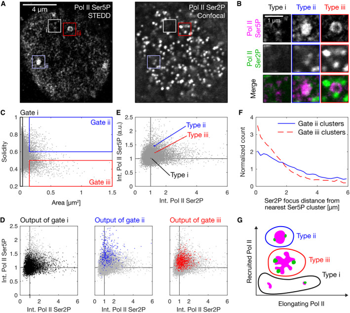
Figure 2
Superu2010resolution microscopy reveals types of cluster morphologies correlating with levels of recruited and elongating RNA polymerase II
Representative nuclear midu2010section obtained by STEDD superu2010resolution microscopy from a fixed sphereu2010stage zebrafish embryo. Pol II Ser5P intensity distributions were obtained by STEDD mic...
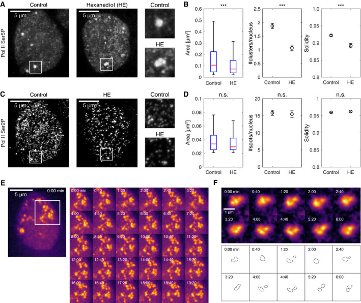
Figure 3
Large clusters of recruited Pol II are partially destabilized by hexanediol treatment, form stable patterns of nonu2010growing domains, and undergo repeated connection and splitting
Representative maximumu2010intensity projection micrographs of nuclei in primary cell cultures of zebrafish embryos, treated for 5u00a0min with control media or 3% 1,6u2010hexanediol (HE), then fixed ...
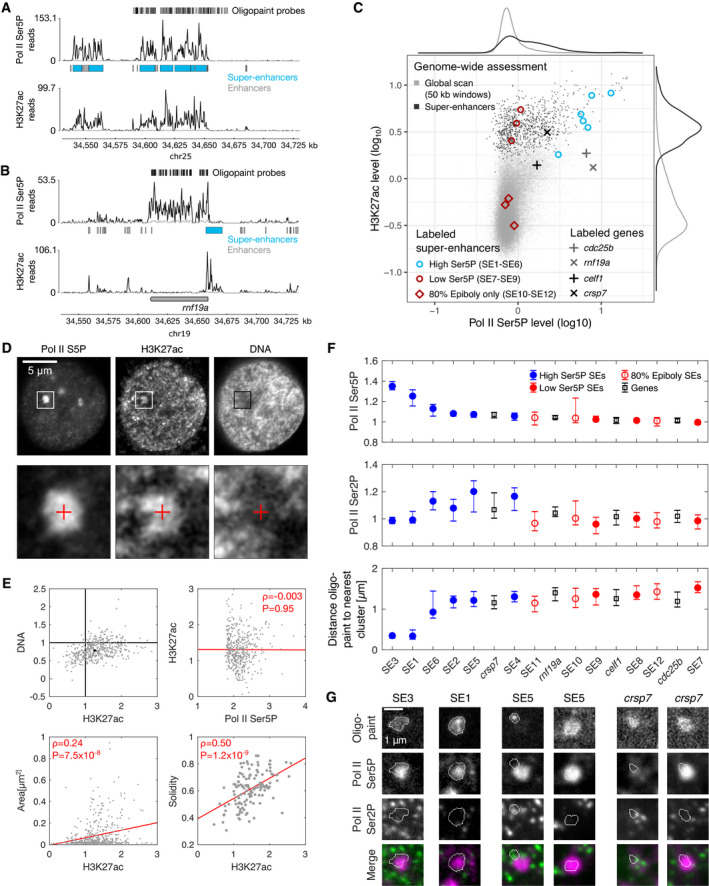
Figure 4
Regulatory chromatin associates with clusters of recruited Pol II
Example view of a genomic region containing a superu2010enhancer (SE3), for an overview of all genomic regions labeled by oligopaint probe sets see Appendixu00a0Fig S8 . Example view of a genomic regi...
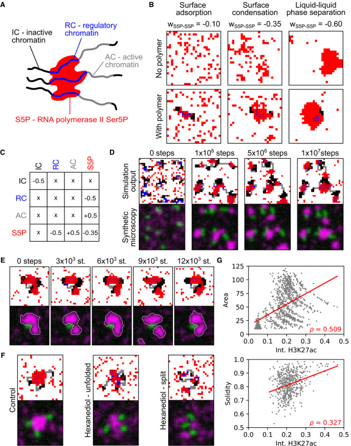
Figure 5
A lattice model exhibits key characteristics of liquidu2010phase condensation with a polymeric subregion as a surface
Sketch of cluster nucleation with the different species involved in the model. Examples of lattice configurations obtained from simulations containing only red particles with increasing selfu2010affin...
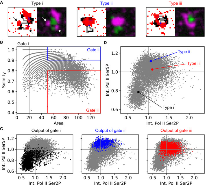
Figure 6
Lattice simulations reproduce the relation between Pol II CTD phosphorylation and cluster morphology
Example lattice configurations for all three cluster morphology cluster types (iu2013iii) are shown as lattice simulation output and the corresponding synthetic microscopy images. Area and solidity of...
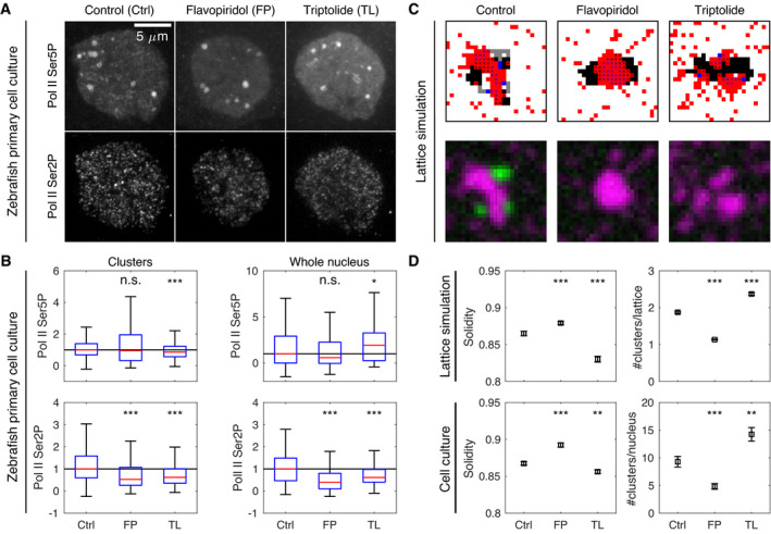
Figure 7
Lattice simulations reproduce the effect of transcription inhibitors on cluster morphology
Representative micrographs showing Pol II Ser5P and Pol II Ser2P in primary cell cultures obtained from zebrafish embryos and treated for 30u00a0min with control media (Ctrl), flavopiridol (FP, 1u00a0...
Figure images are served from the NIH/NLM PubMed Central Open Access Subset or Europe PMC; copyright remains with the publishers and authors.
💬 Discussion
0 commentsNo comments yet. Be the first to start a discussion!
Leave a Comment