Abstract
The simultaneous imaging and manipulating of neural activity could enable the functional dissection of neural circuits. Here we have combined two-photon optogenetics with simultaneous volumetric two-photon calcium imaging to measure and manipulate neural activity in mouse neocortex in vivo in three-dimensions (3D) with cellular resolution. Using a hybrid holographic approach, we simultaneously photostimulate more than 80 neurons over 150 μm in depth in layer 2/3 of the mouse visual cortex, while simultaneously imaging the activity of the surrounding neurons. We validate the usefulness of the method by photoactivating in 3D selected groups of interneurons, suppressing the response of nearby pyramidal neurons to visual stimuli in awake animals. Our all-optical approach could be used as a general platform to read and write neuronal activity.
🔬 Techniques
🔭 Microscopes
💻 Software
✨ Fluorophores
🧪 Sample Preparation
🏭 Microscope Brands
🧪 Reagent Suppliers
🔴 Lasers
📷 Detectors
💻 Software Details
💻 Code & Software
Matlab code for 3D holographic photostimulation and volumetric imaging
Matlab code for 3D holographic photostimulation and volumetric imaging
💾 Data Repositories
🏛️ Research Organizations (ROR)
Affiliated research institutions:
📋 Methods
Microscope design
The optical setup is illustrated in Figure 1A , which is composed of two femtosecond pulse lasers and a custom-modified two-photon laser scanning microscope (Ultima In Vivo, Bruker Corporation, Billerica, Massachusetts). The laser source for imaging is a pulsed Ti:sapphire laser (Chameleon Ultra II, Coherent, Inc., Santa Clara, California). Its wavelength is tuned to 940 nm for GCaMP6s or GCaMP6f imaging or 750 nm for mCherry imaging respectively. The laser power is controlled with a Pockels cell (350–160-BK Pockels cell, 302RM controller, Conoptics, Inc., Danbury, Connecticut). The laser beam is expanded by a 1:3.2 telescopes (f = 125 mm and f = 400 mm) and coupled to an ETL (EL-10-30-C-NIR-LD-MV, Optotune AG, Dietikon, Switzerland) with a clear aperture of 10 mm in diameter. The transmitted beam is rescaled by a 3.2:1 telescope (f = 400 mm and f = 125 mm) and imaged onto a resonant scanner and galvanometric mirror, both located at the conjugate planes to the microscope’s objective pupil. The beam is further scaled by a 1:1.33 telescope before coupled into a scan lens (f = 75 mm), a tube lens (f = 180 mm) and the objective lens (25x N.A. XLPlan N, Olympus Corporation, Tokyo, Japan), yielding an excitation NA ~ 0.45. The laser can also be directed to a non-resonant scanning path (without ETL) where both X and Y scanning are controlled by galvanometric mirrors. The fluorescence signal from the sample is collected through the objective lens and split at a dichroic mirror (HQ575dcxr, 575 nm long pass, Chroma Technology Corp., Bellows Falls, Vermont) to be detected in two bi-alkali photomultiplier tubes, one for each wavelength range. Two different bandpass filters (510/20–2P, and 607/45–2P, Chroma Technology Corp., Bellows Falls, Vermont) are placed in front of the corresponding PMT respectively. The optical path for the photostimulation is largely independent from the imaging, except that they combine at a dichroic mirror (T1030SP, 1030 nm short pass, Chroma Technology Corp., Bellows Falls, Vermont) just before the scan lens, and then share the same optical path. The laser source for photostimulation is a low repetition rate (200 kHz ~ 1 MHz) pulse-amplified laser (Spirit 1040–8, Spectra-physics, Santa Clara, California), operating at 1040 nm wavelength. Its power is controlled by a Pockels cell (1147-4-1064 Pockels cell, 8025RS-H-2KV controller, FastPulse Technology, Saddle Brook, New Jersey). A λ/2 waveplate (AHWP05M-980, Thorlabs, Inc. Newton, New Jersey) is used to rotate the laser polarization so that it is parallel to the active axis of the spatial light modulator (HSP512-1064, 7.68 × 7.68 mm 2 active area, 512 × 512 pixels; Meadowlark Optics, Frederick, Colorado). The beam is expanded by two telescopes (1:1.75, f = 100 mm and f = 175 mm; 1:4, f = 50 mm and f = 200 mm) to fill the active area of the SLM. The reflected beam from the SLM is scaled by a 3:1 telescope (f = 300 mm and f = 100 mm) and imaged onto a set of close-coupled galvanometer mirrors, located at the conjugate plane to the microscope’s objective pupil. A beam block made of a small metallic mask on a thin pellicle is placed at the intermediate plane of this telescope to remove the zeroth-order beam. The photostimulation laser beam reflected from the galvanometer mirrors are then combined with the imaging laser beam at the 1030 nm short pass dichroic mirror. The imaging and photostimulation is controlled by a combination of PrairieView (Bruker Corporation, Billerica, Massachusetts) and custom software ( Yang, 2018 ) running under MATLAB (The Mathworks, Inc. Natick, Massachusetts) on a separate computer. The Matlab program was developed to control the ETL through a data acquisition card (PCIe-6341, National Instrument, Austin, Texas) for volumetric imaging, and the SLM through PCIe interface (Meadowlark Optics, Frederick, Colorado) for holographic photostimulation ( Yang, 2018 ). The two computers are synchronized with shared triggers. At the end of each imaging frame, a signal is received to trigger the change of the drive current (which is converted from a voltage signal from the data acquisition card by a voltage-current converter [LEDD1B, Thorlabs, Inc. Newton, New Jersey]) of the ETL, so the imaging depth is changed for the following frame. The range of the focal length change on sample is ~+90 μm ~ −200 μm (‘+” means longer focal length). The intrinsic imaging frame rate is ~ 30 fps with 512 × 512 pixel image. The effective frame rate is lower as we typically wait 10 ~ 17 ms in between frames to let the ETL fully settle down at the new focal length. The control voltage of the Pockels cell is switched between different imaging planes to maintain image brightness. The typical imaging power is < 50 mW, and could be up to 80 mW for layers deeper than ~ 250 μm. The Matlab programs to control the ETL for volumetric imaging and SLM for holographic photostimulation ( Yang, 2018 ) is available at https://github.com/wjyangGithub/Holographic-Photostimulation-System with a GNU General Public License, version 3 (copy archived at https://github.com/elifesciences-publications/Holographic-Photostimulation-System).
Show full methods section
Microscope design
The optical setup is illustrated in Figure 1A , which is composed of two femtosecond pulse lasers and a custom-modified two-photon laser scanning microscope (Ultima In Vivo, Bruker Corporation, Billerica, Massachusetts). The laser source for imaging is a pulsed Ti:sapphire laser (Chameleon Ultra II, Coherent, Inc., Santa Clara, California). Its wavelength is tuned to 940 nm for GCaMP6s or GCaMP6f imaging or 750 nm for mCherry imaging respectively. The laser power is controlled with a Pockels cell (350–160-BK Pockels cell, 302RM controller, Conoptics, Inc., Danbury, Connecticut). The laser beam is expanded by a 1:3.2 telescopes (f = 125 mm and f = 400 mm) and coupled to an ETL (EL-10-30-C-NIR-LD-MV, Optotune AG, Dietikon, Switzerland) with a clear aperture of 10 mm in diameter. The transmitted beam is rescaled by a 3.2:1 telescope (f = 400 mm and f = 125 mm) and imaged onto a resonant scanner and galvanometric mirror, both located at the conjugate planes to the microscope’s objective pupil. The beam is further scaled by a 1:1.33 telescope before coupled into a scan lens (f = 75 mm), a tube lens (f = 180 mm) and the objective lens (25x N.A. XLPlan N, Olympus Corporation, Tokyo, Japan), yielding an excitation NA ~ 0.45. The laser can also be directed to a non-resonant scanning path (without ETL) where both X and Y scanning are controlled by galvanometric mirrors. The fluorescence signal from the sample is collected through the objective lens and split at a dichroic mirror (HQ575dcxr, 575 nm long pass, Chroma Technology Corp., Bellows Falls, Vermont) to be detected in two bi-alkali photomultiplier tubes, one for each wavelength range. Two different bandpass filters (510/20–2P, and 607/45–2P, Chroma Technology Corp., Bellows Falls, Vermont) are placed in front of the corresponding PMT respectively. The optical path for the photostimulation is largely independent from the imaging, except that they combine at a dichroic mirror (T1030SP, 1030 nm short pass, Chroma Technology Corp., Bellows Falls, Vermont) just before the scan lens, and then share the same optical path. The laser source for photostimulation is a low repetition rate (200 kHz ~ 1 MHz) pulse-amplified laser (Spirit 1040–8, Spectra-physics, Santa Clara, California), operating at 1040 nm wavelength. Its power is controlled by a Pockels cell (1147-4-1064 Pockels cell, 8025RS-H-2KV controller, FastPulse Technology, Saddle Brook, New Jersey). A λ/2 waveplate (AHWP05M-980, Thorlabs, Inc. Newton, New Jersey) is used to rotate the laser polarization so that it is parallel to the active axis of the spatial light modulator (HSP512-1064, 7.68 × 7.68 mm 2 active area, 512 × 512 pixels; Meadowlark Optics, Frederick, Colorado). The beam is expanded by two telescopes (1:1.75, f = 100 mm and f = 175 mm; 1:4, f = 50 mm and f = 200 mm) to fill the active area of the SLM. The reflected beam from the SLM is scaled by a 3:1 telescope (f = 300 mm and f = 100 mm) and imaged onto a set of close-coupled galvanometer mirrors, located at the conjugate plane to the microscope’s objective pupil. A beam block made of a small metallic mask on a thin pellicle is placed at the intermediate plane of this telescope to remove the zeroth-order beam. The photostimulation laser beam reflected from the galvanometer mirrors are then combined with the imaging laser beam at the 1030 nm short pass dichroic mirror. The imaging and photostimulation is controlled by a combination of PrairieView (Bruker Corporation, Billerica, Massachusetts) and custom software ( Yang, 2018 ) running under MATLAB (The Mathworks, Inc. Natick, Massachusetts) on a separate computer. The Matlab program was developed to control the ETL through a data acquisition card (PCIe-6341, National Instrument, Austin, Texas) for volumetric imaging, and the SLM through PCIe interface (Meadowlark Optics, Frederick, Colorado) for holographic photostimulation ( Yang, 2018 ). The two computers are synchronized with shared triggers. At the end of each imaging frame, a signal is received to trigger the change of the drive current (which is converted from a voltage signal from the data acquisition card by a voltage-current converter [LEDD1B, Thorlabs, Inc. Newton, New Jersey]) of the ETL, so the imaging depth is changed for the following frame. The range of the focal length change on sample is ~+90 μm ~ −200 μm (‘+” means longer focal length). The intrinsic imaging frame rate is ~ 30 fps with 512 × 512 pixel image. The effective frame rate is lower as we typically wait 10 ~ 17 ms in between frames to let the ETL fully settle down at the new focal length. The control voltage of the Pockels cell is switched between different imaging planes to maintain image brightness. The typical imaging power is < 50 mW, and could be up to 80 mW for layers deeper than ~ 250 μm. The Matlab programs to control the ETL for volumetric imaging and SLM for holographic photostimulation ( Yang, 2018 ) is available at https://github.com/wjyangGithub/Holographic-Photostimulation-System with a GNU General Public License, version 3 (copy archived at https://github.com/elifesciences-publications/Holographic-Photostimulation-System).
SLM hologram and characterization
The phase hologram on the SLM, ϕ ( u , v ) , can be expressed as: (1) ϕ ( u , v ) = p h a s e { ∑ i = 1 M A i e 2 π j { x i u + y i v + [ Z 2 0 ( u , v ) C 2 0 ( z i ) + Z 4 0 ( u , v ) C 4 0 ( z i ) + Z 6 0 ( u , v ) C 6 0 ( z i ) ] } } where [ x i , y i , z i ] ( i = 1,2… M ) is the coordinate of the cell body centroid ( M targeted cells in total), and A i is the electrical field weighting coefficient for the i th target (which controls the laser power it receives). Z m 0 ( u , v ) and C m 0 ( z i ) are the Zernike polynomials and Zernike coefficients, respectively, which sets the defocusing and compensates the first-order and second-order spherical aberration due to defocusing. Their expressions are shown in Table 1 . The hologram can also be generated by 3D Gerchberg-Saxton algorithm, with additional steps to incorporate spherical aberration compensation. We adapt Equation (1) as a simpler method. For the experiments in Figure 2 , and Figure 2—figure supplement 1 , the Gerchberg-Saxton algorithm is used to generate a disk with a diameter similar to the neurons. 10.7554/eLife.32671.015 Table 1. Expression of Zernike polynomials and Zernike coefficients in Equation (1) . Defocus Zernike polynomials Z 2 0 ( u , v ) = 3 [ 2 ( u 2 + v 2 ) − 1 ] Zernike coefficients C 2 0 ( z ) = n k z sin 2 α 8 π 3 ( 1 + 1 4 sin 2 α + 9 80 sin 4 α + 1 16 sin 6 α + ⋅ ⋅ ⋅ ) First-order spherical aberration Zernike polynomials Z 4 0 ( u , v ) = 5 [ 6 ( u 2 + v 2 ) 2 − 6 ( u 2 + v 2 ) + 1 ] Zernike coefficients C 4 0 ( z ) = n k z sin 4 α 96 π 5 ( 1 + 3 4 sin 2 α + 15 18 sin 4 α + ⋅ ⋅ ⋅ ) Second-order spherical aberration Zernike polynomials Z 6 0 ( u , v ) = 7 [ 20 ( u 2 + v 2 ) 3 − 30 ( u 2 + v 2 ) 2 + 12 ( u 2 + v 2 ) − 1 ] Zernike coefficients C 6 0 ( z ) = n k z sin 6 α 640 π 7 ( 1 + 5 4 sin 2 α + ⋅ ⋅ ⋅ ) n , refractive index of media between the objective and sample; k , the wavenumber; z , the axial shift of the focus plane in the sample; u , v , coordinates on the SLM phase mask; n sin α , the NA of the objective. To match the defocusing length set in SLM with the actual defocusing length, we adjusted the ‘effective N.A.’ in the Zernike coefficients following the calibration procedure described in Ref. ( Yang et al., 2016 ). To register the photostimulation beam’s targeting coordinate in lateral directions, we projected 2D holographic patterns to burn spots on the surface of an autofluorescent plastic slide and visualized them by the imaging laser. An affine transformation can be extracted to map the coordinates. We repeated this registration for every 25 μm defocusing depth on the sample, and applied a linear interpolation to the depths in between. An alternative method to register the targeting coordinate is to set the photostimulation laser in imaging mode, actuate the SLM for different lateral deflection, and extract the transform matrix from the acquired images and that acquired from the imaging laser. To characterize the lateral registration error, we actuated the SLM and burned spots on the surface of an autofluorescent plastic slide across a field of view of 240 μm x 240 μm with a 7 × 7 grid pattern. We then imaged the spots pattern with the imaging laser and measured the registration error. This was repeated for different SLM focal depths. To characterize the axial registration error, we used the photostimulation laser to image a slide with quantum dots sample. The SLM was set at different focal depths, and a z-stack was acquired for each setting to measure the actual defocus and thus the axial registration error. In all these registration and characterization procedures, we used water as the media between the objective and the sample, and we kept the focus of the photostimulation laser at the sample surface by translating the microscope stage axially. We note that the refractive index of the brain tissue is slightly different from that of water (~2%), and this could cause an axial shift of the calibration. This could be corrected in the Zernike coefficients. In practice, we found this effect is negligible, as the typical focal shift by the SLM is relatively small (
📊 Figures
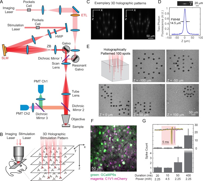
Figure 1.
Two-photon imaging and photostimulation microscope.
( A ) Dual two-photon excitation microscope setup. HWP, half-wave plate; ZB, zeroth-order beam block; SLM, spatial light modulator; ETL, electrically tunable lens; PMT, photomultiplier tube. ( B ) Sch...
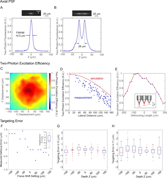
Figure 1u2014figure supplement 1.
System characterization of the spatial light modulator (SLM) in the 3D microscope.
( A ) Measured point spread function (PSF) in the axial (z) direction for two-photon excitation. The FWHM is 14.5 u03bcm, corresponding to an NAu00a0~u00a00.35. ( B ) Measured axial profile of a two-p...
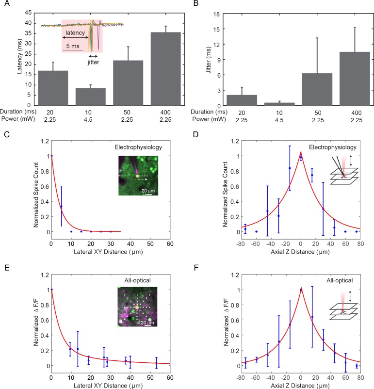
Figure 1u2014figure supplement 2.
Characterization and spatial resolution of photostimulation.
( A u2013 B ) Latency ( A ) and jitter ( B ) of target pyramidal cells in layer 2/3 of mouse V1 evoked by photostimulation with different spiral duration and average laser power (3 cells in each condi...
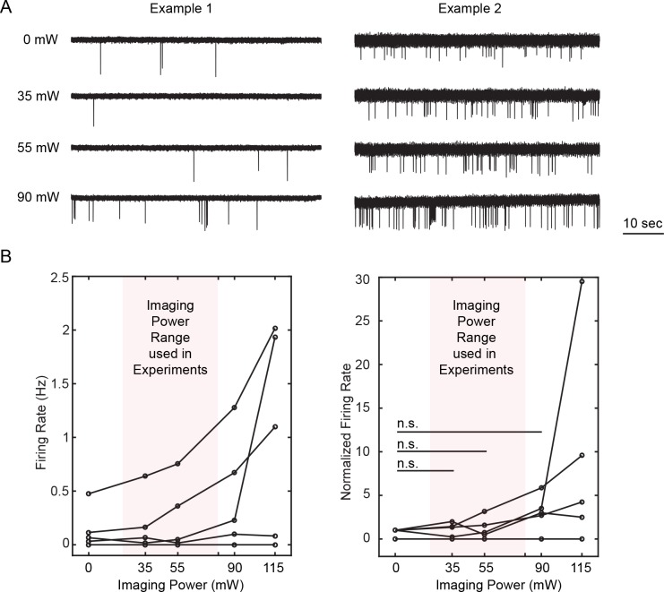
Figure 1u2014figure supplement 3.
Cross talk from imaging into photostimulation.
Activities of neurons in layer 2/3 of mice V1 were recorded by cell-attached electrophysiology while the whole field was being scanned by the imaging laser (940 nm) at an FOV of 240 u00d7 240 u03bcm 2...
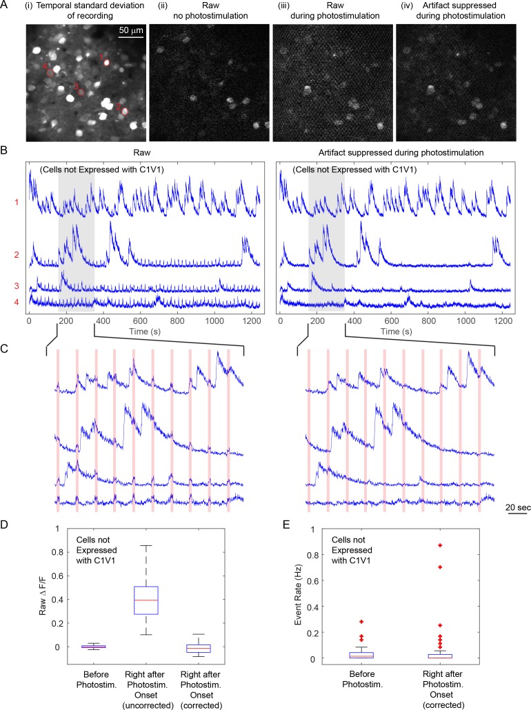
Figure 1u2014figure supplement 4.
Cross talk from photostimulation into imaging.
This example represents one of the worst cross talk situation: the bright GCaMP6s signal, the relatively strong photostimulation power (60 mW) and its long duration (2.8 s) render a strong photostimul...
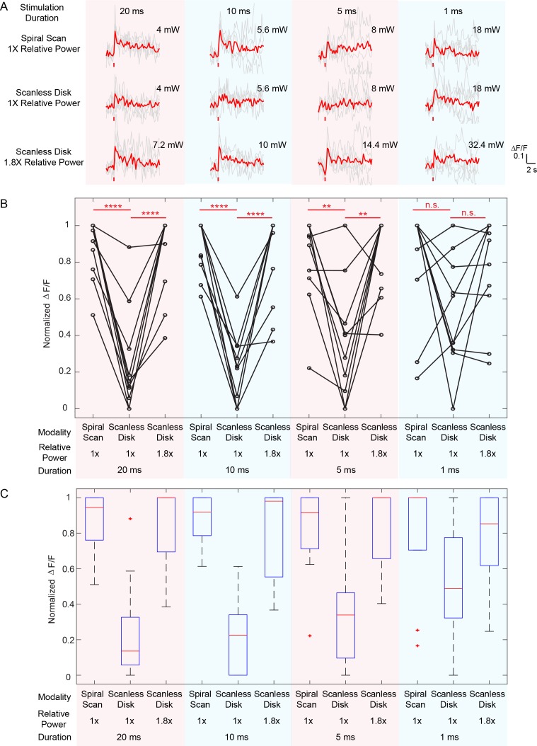
Figure 2.
Comparison between spiral scan and scanless holographic approaches for photostimulation.
In the scanning approach, the laser spot is spirally scanned over the cell body; in the scanless approach, a disk pattern (~12 u03bcm in diameter) is generated by the SLM, covering the entire cell bod...
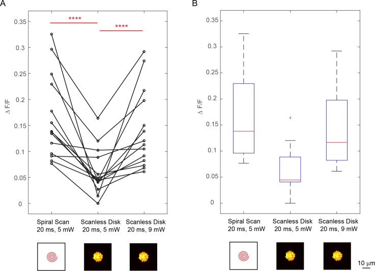
Figure 2u2014figure supplement 1.
Comparison between spiral scan and scanless holographic approaches for photostimulation.
In the scanning approach, the laser spot is spirally scanned over the cell body; in the scanless approach, a disk pattern (~12 u03bcm in diameter) is generated by the SLM, covering the entire cell bod...
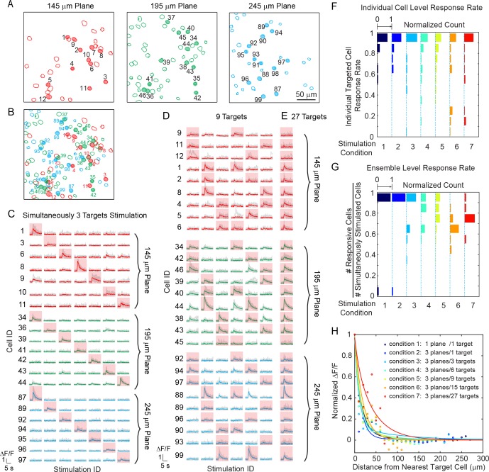
Figure 3.
Simultaneous holographicu00a0photostimulation of pyramidal cells in vivo.
( A ) Contour maps showing the spatial location of the cells in three individual planes inu00a0mouseu00a0V1u00a0(145 u03bcm, 195 u03bcm, and 245 u03bcm from pial surface). Cells with shaded color are ...
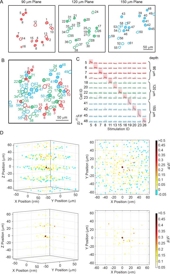
Figure 3u2014figure supplement 1.
Sequential photostimulation of individual pyramidal cells in layer 2/3 from mouse V1 in vivo.
( A ) Contour maps showing the spatial location of the cells in three individual planes inu00a0mouseu00a0V1u00a0(90 u03bcm, 120 u03bcm, and 150 u03bcm from pial surface). Cells with shaded color are t...
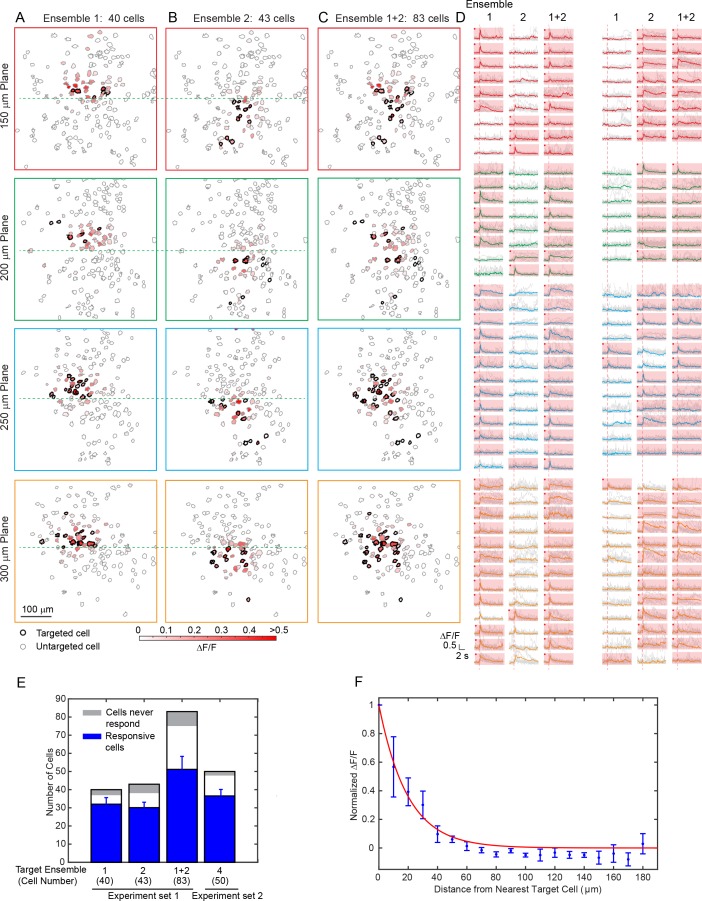
Figure 4.
Large scale photostimulation of pyramidal cells in layer 2/3 of V1 in awake mice.
( A ~ C ) Simultaneous photostimulation of 40 cells, 43 cells and 83 cells across four planes inu00a0mouseu00a0V1u00a0(150 u03bcm, 200 u03bcm, 250 u03bcm and 300 u03bcm from pial surface, with an imag...
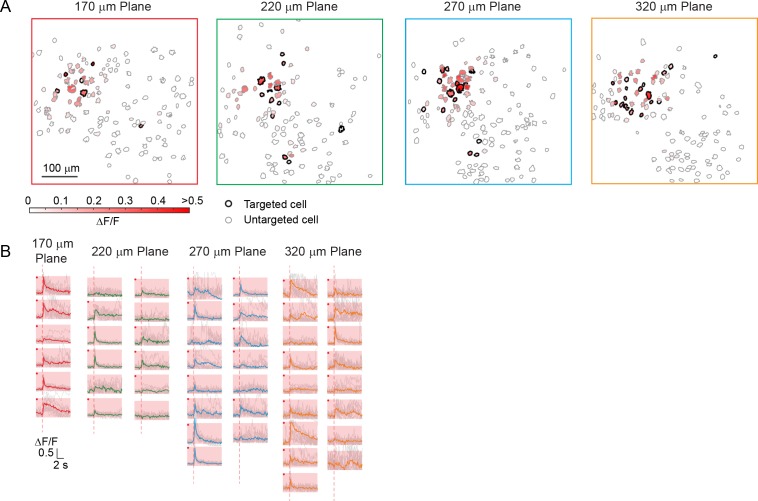
Figure 4u2014figure supplement 1.
Simultaneous photostimulation of 50 pyramidal cells in layer 2/3 of V1 in awake mice.
( A ) Contour maps showing the spatial location of the cells acrossu00a0four individual planes inu00a0mouseu00a0V1u00a0(170 u03bcm, 220 u03bcm, 270 u03bcm and 320 u03bcm from pial surface). Cells with...
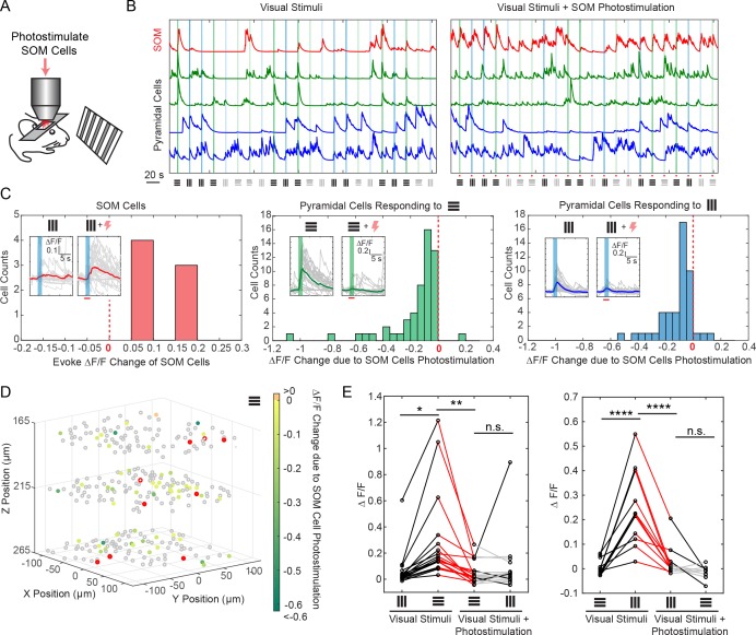
Figure 5.
Selective photostimulation of SOM interneurons suppresses visual response of pyramidal cells in awake mice.
( A ) Experiment paradigm where the SOM cells were photostimulated when the mouse received drifting grating visual stimulation. ( B ) Normalized calcium traces (u0394F/F) of representative targeted SO...
Figure images are served from the NIH/NLM PubMed Central Open Access Subset or Europe PMC; copyright remains with the publishers and authors.
💬 Discussion
0 commentsNo comments yet. Be the first to start a discussion!
Leave a Comment