Abstract
Abstract Association areas in neocortex encode novel stimulus-outcome relationships, but the principles of their engagement during task learning remain elusive. Using chronic wide-field calcium imaging, we reveal two phases of spatiotemporal refinement of layer 2/3 cortical activity in mice learning whisker-based texture discrimination in the dark. Even before mice reach learning threshold, association cortex—including rostro-lateral (RL), posteromedial (PM), and retrosplenial dorsal (RD) areas—is generally suppressed early during trials (between auditory start cue and whisker-texture touch). As learning proceeds, a spatiotemporal activation sequence builds up, spreading from auditory areas to RL immediately before texture touch (whereas PM and RD remain suppressed) and continuing into barrel cortex, which eventually efficiently discriminates between textures. Additional correlation analysis substantiates this diverging learning-related refinement within association cortex. Our results indicate that a pre-learning phase of general suppression in association cortex precedes a learning-related phase of task-specific signal flow enhancement.
🔬 Techniques
✨ Fluorophores
🧪 Sample Preparation
🏭 Microscope Brands
🧪 Reagent Suppliers
📷 Detectors
💻 Software Details
💾 Data Repositories
🏛️ Research Organizations (ROR)
Affiliated research institutions:
📋 Methods
Animals and surgical procedures
Methods were carried out according to the guidelines of the Veterinary Office of Switzerland and following approval by the Cantonal Veterinary Office in Zurich. A total of 7 adult male mice (1-4 months old) were used in this study. These mice were triple transgenic Rasgrf2-2A-dCre;CamK2a-tTA;TITL-GCaMP6f animals, expressing GCaMP6f in excitatory neocortical layer 2/3 neurons 11 . To generate triple transgenic animals, double transgenic mice carrying CamK2a-Tta 62 and TITL-GCaMP6f 63 were crossed with a Rasgrf2-2A-dCre line ( 64 ; individual lines are available from The Jackson Laboratory as JAX# 016198, JAX#024103, and JAX# 022864, respectively). The Rasgrf2-2A-dCre;CamK2a-tTA;TITL-GCaMP6f line contains a tet-off system, by which transgene expression can be suppressed upon doxycycline treatment 65 , 66 . However, doxycycline treatment is not necessary in these animals, since the Rasgrf2-2A-dCre line holds an inducible system of its own, given that the destabilized Cre (dCre) expressed under the control of the Rasgrf2-2A promoter needs to be stabilized by trimethoprim (TMP) to be fully functional. TMP (Sigma T7883) was reconstituted in Dimethyl sulfoxide (DMSO, Sigma 34869) at a saturation level of 100 mg/ml, freshly prepared for each experiment. For TMP induction, mice were given a single intraperitoneal injection (150 µg TMP/g body weight; 29 g needle; 3–5 days post-surgery), diluted in 0.9% saline solution. We used an intact skull preparation 67 for chronic wide-field calcium imaging of neocortical activity 11 . Mice were anesthetized with 2% isoflurane (in pure O 2 ) and body temperature was maintained at 37 °C. We applied local analgesia (lidocaine 1%), exposed and cleaned the skull, and removed some muscles to access the entire dorsal surface of the left hemisphere (Fig. 2a ; ~6 × 8 mm 2 from ~3 mm anterior to bregma to ~1 mm posterior to lambda; from the midline to at least 5 mm laterally). We built a wall around the hemisphere with adhesive material (iBond; UV-cured) and dental cement “worms” (Charisma). Then, we applied transparent dental cement homogenously over the imaging field (Tetric EvoFlow T1). Finally, a metal post for head fixation was glued on the back of the right hemisphere. This minimally invasive preparation enabled high-quality chronic imaging with high success rate. Texture discrimination task Mice were trained on a go/no-go discrimination task (Fig. 1a ) using a data acquisition interface (USB-6008; National Instruments) and custom-written LabVIEW software (National Instruments 27 ). Each trial started with an auditory cue (stimulus cue; 2 beeps at 2 kHz, 100-ms duration with 50-ms interval), signaling the approach of either two types of sandpapers (grit size P100: rough texture; P1200: smooth texture; 3M) to the mouse’s whiskers as ‘go’ or ‘no-go’ textures (Fig. 1a ; pseudo-randomly presented with no more than three repetitions). Sandpapers were mounted onto panels attached to a stepper motor (T-NM17A04; Zaber) mounted onto a motorized linear stage (T-LSM100A; Zaber) to move textures in and out of reach of whiskers. The texture stayed in touch with the whiskers for 2 s, and then it was moved out after which an additional auditory cue (response cue; 4 beeps at 4 kHz, 50-ms duration with 25-ms interval) signaled the start of a 2-s response period. The stimulus and response cues were identical in both textures. A water reward (~3 µL) was given to the mouse for licking for the go texture only after the response cue (‘hit’), i.e. for the first correct lick during the response period (Fig. 1e ; lick were detected using a piezo sensor). Punishment with white noise was given for licking for the no-go texture (‘false alarms’; FA). Licking before the response cue was neither rewarded nor punished. Reward and punishment were omitted when mice withheld licking for the no-go (‘correct-rejections’, CR) or go (‘Misses’) textures. The licking detector remained in a fixed and reachable position throughout the entire trial. Note that the auditory tones merely served as cues defining the temporal trial structure, but had no predictive power with respect to go or no-go condition. The first auditory tone signaled the trial-start and thus predicted the upcoming arrival of the texture as the task-relevant stimulus, whereas the second auditory tone indicated the availability of a water reward in the go trials. Licking before the response cue was allowed and did not lead to punishment or early reward. Training and performance Five mice were trained to lick for the P100 texture (mice #1-4 and 7) and 2 mice were trained to lick for the P1200 texture (mice #5 and 6). Mice were first handled and accustomed to head fixation before starting water scheduling. Before imaging began mice were conditioned to lick for reward after the go texture (presented within a similar trial structure as the task itself). Imaging began only after mice reliably licked for the response cue (typically after the first day; 200–400 trials). On the first day of imaging, mice were presented with the ‘go’ texture and after 50 trials the ‘no-go’ texture was gradually introduced (starting from 10% and increasing by 10% approximately every 50 trials 68 ) until reaching 50% probability for the no-go texture by the end of the day. During the second day, most mice continuously licked for both textures (Supplementary Fig. 2 ). Thus after around 100 trials, we increased no-go probability to 80% and waited for mice to perform three continuous CR trials before returning to 50% probability. This was done for several times until mice increased their performance, specifically withheld licking for the no-go texture. In mice that still continued to lick for both textures we additionally repeated the wrong response until a correct response. In all mice, a 50% protocol was presented with no repetitions as soon as they reached expert level (d′ > 1.5). 6 out of the 7 mice learned the task within 3–4 days after around a thousand trials (Fig. 1d ; Supplementary Fig. 2 ). Mouse #7 learned the task within 10 days. An effort was made to maintain a constant position of the texture and cameras across imaging days in order to maintain similar stimulation and imaging parameters.
Show full methods section
Animals and surgical procedures
Methods were carried out according to the guidelines of the Veterinary Office of Switzerland and following approval by the Cantonal Veterinary Office in Zurich. A total of 7 adult male mice (1-4 months old) were used in this study. These mice were triple transgenic Rasgrf2-2A-dCre;CamK2a-tTA;TITL-GCaMP6f animals, expressing GCaMP6f in excitatory neocortical layer 2/3 neurons 11 . To generate triple transgenic animals, double transgenic mice carrying CamK2a-Tta 62 and TITL-GCaMP6f 63 were crossed with a Rasgrf2-2A-dCre line ( 64 ; individual lines are available from The Jackson Laboratory as JAX# 016198, JAX#024103, and JAX# 022864, respectively). The Rasgrf2-2A-dCre;CamK2a-tTA;TITL-GCaMP6f line contains a tet-off system, by which transgene expression can be suppressed upon doxycycline treatment 65 , 66 . However, doxycycline treatment is not necessary in these animals, since the Rasgrf2-2A-dCre line holds an inducible system of its own, given that the destabilized Cre (dCre) expressed under the control of the Rasgrf2-2A promoter needs to be stabilized by trimethoprim (TMP) to be fully functional. TMP (Sigma T7883) was reconstituted in Dimethyl sulfoxide (DMSO, Sigma 34869) at a saturation level of 100 mg/ml, freshly prepared for each experiment. For TMP induction, mice were given a single intraperitoneal injection (150 µg TMP/g body weight; 29 g needle; 3–5 days post-surgery), diluted in 0.9% saline solution. We used an intact skull preparation 67 for chronic wide-field calcium imaging of neocortical activity 11 . Mice were anesthetized with 2% isoflurane (in pure O 2 ) and body temperature was maintained at 37 °C. We applied local analgesia (lidocaine 1%), exposed and cleaned the skull, and removed some muscles to access the entire dorsal surface of the left hemisphere (Fig. 2a ; ~6 × 8 mm 2 from ~3 mm anterior to bregma to ~1 mm posterior to lambda; from the midline to at least 5 mm laterally). We built a wall around the hemisphere with adhesive material (iBond; UV-cured) and dental cement “worms” (Charisma). Then, we applied transparent dental cement homogenously over the imaging field (Tetric EvoFlow T1). Finally, a metal post for head fixation was glued on the back of the right hemisphere. This minimally invasive preparation enabled high-quality chronic imaging with high success rate. Texture discrimination task Mice were trained on a go/no-go discrimination task (Fig. 1a ) using a data acquisition interface (USB-6008; National Instruments) and custom-written LabVIEW software (National Instruments 27 ). Each trial started with an auditory cue (stimulus cue; 2 beeps at 2 kHz, 100-ms duration with 50-ms interval), signaling the approach of either two types of sandpapers (grit size P100: rough texture; P1200: smooth texture; 3M) to the mouse’s whiskers as ‘go’ or ‘no-go’ textures (Fig. 1a ; pseudo-randomly presented with no more than three repetitions). Sandpapers were mounted onto panels attached to a stepper motor (T-NM17A04; Zaber) mounted onto a motorized linear stage (T-LSM100A; Zaber) to move textures in and out of reach of whiskers. The texture stayed in touch with the whiskers for 2 s, and then it was moved out after which an additional auditory cue (response cue; 4 beeps at 4 kHz, 50-ms duration with 25-ms interval) signaled the start of a 2-s response period. The stimulus and response cues were identical in both textures. A water reward (~3 µL) was given to the mouse for licking for the go texture only after the response cue (‘hit’), i.e. for the first correct lick during the response period (Fig. 1e ; lick were detected using a piezo sensor). Punishment with white noise was given for licking for the no-go texture (‘false alarms’; FA). Licking before the response cue was neither rewarded nor punished. Reward and punishment were omitted when mice withheld licking for the no-go (‘correct-rejections’, CR) or go (‘Misses’) textures. The licking detector remained in a fixed and reachable position throughout the entire trial. Note that the auditory tones merely served as cues defining the temporal trial structure, but had no predictive power with respect to go or no-go condition. The first auditory tone signaled the trial-start and thus predicted the upcoming arrival of the texture as the task-relevant stimulus, whereas the second auditory tone indicated the availability of a water reward in the go trials. Licking before the response cue was allowed and did not lead to punishment or early reward. Training and performance Five mice were trained to lick for the P100 texture (mice #1-4 and 7) and 2 mice were trained to lick for the P1200 texture (mice #5 and 6). Mice were first handled and accustomed to head fixation before starting water scheduling. Before imaging began mice were conditioned to lick for reward after the go texture (presented within a similar trial structure as the task itself). Imaging began only after mice reliably licked for the response cue (typically after the first day; 200–400 trials). On the first day of imaging, mice were presented with the ‘go’ texture and after 50 trials the ‘no-go’ texture was gradually introduced (starting from 10% and increasing by 10% approximately every 50 trials 68 ) until reaching 50% probability for the no-go texture by the end of the day. During the second day, most mice continuously licked for both textures (Supplementary Fig. 2 ). Thus after around 100 trials, we increased no-go probability to 80% and waited for mice to perform three continuous CR trials before returning to 50% probability. This was done for several times until mice increased their performance, specifically withheld licking for the no-go texture. In mice that still continued to lick for both textures we additionally repeated the wrong response until a correct response. In all mice, a 50% protocol was presented with no repetitions as soon as they reached expert level (d′ > 1.5). 6 out of the 7 mice learned the task within 3–4 days after around a thousand trials (Fig. 1d ; Supplementary Fig. 2 ). Mouse #7 learned the task within 10 days. An effort was made to maintain a constant position of the texture and cameras across imaging days in order to maintain similar stimulation and imaging parameters.
Wide-field calcium imaging
We used a wide-field approach to image large parts of the dorsal cortex while mice learned to perform the task 11 . A sensitive CMOS camera (Hamamatsu Orca Flash 4.0) was mounted on top of a dual objective setup. Two objectives (Navitar; top objective: D-5095, 50 mm f0.95; bottom objective inverted: D-2595, 25 mm f0.95) were interfaced with a dichroic (510 nm; AHF; Beamsplitter T510LPXRXT) filter cube (Thorlabs). This combination allowed a ~9-mm field-of-view, covering most of the dorsal cortex of the hemisphere contralateral to texture presentation. Blue LED light (Thorlabs; M470L3) was guided through an excitation filter (480/40 nm BrightLine HC), a diffuser, collimated, reflected from the dichroic mirror, and focused through the bottom objective ~100 µm below the blood vessels. Green light emitted from the preparation passed through both objectives and an emission filter (514/30 nm BrightLine HC) before reaching the camera. The total power of blue light on the preparation was 0.05; Mann–Whitney U -test; n = 7 mice). We note that the first touch occurred mostly (but not exclusively) in the pre-period from −1 to −0.5 relative to texture stop.
Calculation of curves across learning
Trials were binned ( n = 50 trials with no overlap) across learning and the performance (defined as d′ = Z (Hit/(Hit+Miss)) – Z (FA/(FA + CR)) where Z denotes the inverse of the cumulative distribution function) was calculated for each bin. Next, each behavioral learning curve was fitted with a sigmoid function 1 documentclass[12pt]{minimal} usepackage{amsmath} usepackage{wasysym} usepackage{amsfonts} usepackage{amssymb} usepackage{amsbsy} usepackage{mathrsfs} usepackage{upgreek} setlength{oddsidemargin}{-69pt} begin{document}$$S(t) = afrac{1}{{1 + e^{frac{{ - (t - b)}}{c}}}}$$end{document} S ( t ) = a 1 1 + e − ( t − b ) c Where a denotes the amplitude, b the time point (in trial numbers) of the inflection point, and c the steepness of the sigmoid. A d′ = 1.5 was defined as the threshold and mice were ordered based on the trial number at which they crossed threshold (i.e. learning threshold; Fig. 1g ). Varying the d′ threshold maintained the order of the mice based on their learning threshold (see Fig. 1f ). To compare the behavioral learning curve with other behavioral parameters and neuronal activity, we similarly grouped trials and separated them based on the texture type, i.e. hit and miss trials were grouped into the go texture trials; CR and FA trials were grouped into the no-go texture trials. Our main focus in this study was on the go texture (presented in Figs. 2 – 6 ). Therefore, stimulus identity was kept similar across learning. However, results were maintained when considering only the no-go texture trials. Only in Fig. 7 we compare between go and no-go textures to calculate discrimination power. Next, we can present the dynamics of a behavioral parameter (i.e. body movement, whisking envelope or licking probability) or cortical area activity (averaged over pixels) in two-dimensional temporal spaces where the x -axis is the trial temporal structure (i.e. trial dimension) and the y -axis is the learning profile across trials and days (i.e. learning dimension; for examples see Figs. 2a, e, i and 3c (top)). From this 2D temporal space we could average across trials of the learning dimension, e.g. during naïve and expert states (for example see Figs. 2b, f, j and 3c (middle)). Alternatively, we can average across time frames within the trial dimension, to obtain a response curve across learning for a specific time period (i.e. cue-, pre-, or stim-period; additionally smoothed with a Gaussian kernel (2 σ = 9) and fitted with a sigmoid function; for example see Figs. 2c, g, k and 3c (bottom)). Thus we are able to obtain a curve across learning for a specific area or behavioral parameter which are comparable to the behavioral learning curve of the mouse. The sigmoid fits of the response curves from different cortical areas were normalized between 0 and 1 in order to compare between response curves of different areas. This was done mainly because of the different activation ranges across learning for each area. Non-normalized learning curves are presented in Supplementary Fig. 7 . In an additional analysis we also fitted each response curve for all areas and time periods with a double sigmoid fit in order to fit both the initial suppression and the later enhancement that was present in some curves (e.g. Fig. 4d ; Supplementary Fig. 9 ): 2 documentclass[12pt]{minimal} usepackage{amsmath} usepackage{wasysym} usepackage{amsfonts} usepackage{amssymb} usepackage{amsbsy} usepackage{mathrsfs} usepackage{upgreek} setlength{oddsidemargin}{-69pt} begin{document}$${mathrm{d}}(t) = a1left( {1 - frac{1}{{1 + e^{left( {frac{{ - (t - b1)}}{{c1}}} right)}}}} right) + a2left( {1 + frac{1}{{1 + e^{left( {frac{{ - left( {t - b2} right)}}{{c2}}} right)}}}} right) + d$$end{document} d ( t ) = a 1 1 − 1 1 + e − ( t − b 1 ) c 1 + a 2 1 + 1 1 + e − t − b 2 c 2 + d with a 1 and a 2 as amplitudes, b 1 and b 2 as inflection points (in trial numbers), and c 1 and c 2 as steepness parameters of the descending and ascending sigmoid, respectively. d is a baseline parameter, which was set to the minimum value of a curve. Thus, for each area we could quantify the amount (amplitude) and timing (latency) of both suppression and enhancement during each time period relative to the learning threshold. Finally, to quantify the enhancement-suppression ratio we calculated the modulation index (MI) as 3 documentclass[12pt]{minimal} usepackage{amsmath} usepackage{wasysym} usepackage{amsfonts} usepackage{amssymb} usepackage{amsbsy} usepackage{mathrsfs} usepackage{upgreek} setlength{oddsidemargin}{-69pt} begin{document}$${mathrm{MI}} = frac{{a2 - a1}}{{a2 + a1}}$$end{document} MI = a 2 − a 1 a 2 + a 1 ranging from −1 and 1, with positive values indicating more enhancement, negative values indicating more suppression, and near zero values indicating similar amounts of suppression and enhancement. Calculating learning maps and seep maps To study the relationship between the behavioral learning curve and the learning curves of all pixels we calculated a ‘learning map’ (Fig. 5 ). This was done by calculating the correlation coefficient (r) between the behavioral learning curve of the mouse and the learning-related Δ F / F changes of each pixel (Fig. 5a ). This can be done for a specific time period (i.e. cue-, pre- or stim-period; Fig. 5a, b ) or for each time frame (Fig. 5c ). To calculate the relationship between the learning-related Δ F / F changes of a specific area (i.e. seed) and the learning-related Δ F / F changes of all pixels we calculated a seed correlation map (Fig. 6 ). This was done similarly to the learning map by only substituting the behavioral learning curve with the learning-related Δ F / F changes of the desired area (defined as the seed area; Fig. 6a ). We chose seed areas to be RL, PM, and RD which were of the highest interest based on previous analysis and best represent the main trends of neuronal changes during learning. A full correlation matrix between all learning curves is presented in Supplementary Fig. 10 . Discrimination power between go and no-go texture To measure how well could neuronal populations discriminate between go and no-go textures, we calculated a receiver operating characteristics (ROC) curve and calculated its area under the curve (AUC; with a value of 0.5 indicating no discrimination power). This can be done for each pixel (Fig. 7e ), each area (Fig. 7d ), each time frame (Fig. 7b ), and across learning (Fig. 7f ). We put our main focus on the stim-period when the texture touched the whiskers. To calculate significance, we calculated the sample distribution by trial shuffling between go and no-go textures ( n = 100 iterations). Exceeding mean ± 2 s.d. of the sample distribution is defined as significant (Fig. 7b ).
Statistical analysis
In general, non-parametric two-tailed statistical tests were used, Mann–Whitney U -test to compare between two medians from two populations or the Wilcoxon signed-rank test to compare a population’s median to zero (or between two paired populations). Multiple group correction was used when comparing between more than two groups. Reporting summary Further information on research design is available in the Nature Research Reporting Summary linked to this article.
Animals and surgical procedures
Methods were carried out according to the guidelines of the Veterinary Office of Switzerland and following approval by the Cantonal Veterinary Office in Zurich. A total of 7 adult male mice (1-4 months old) were used in this study. These mice were triple transgenic Rasgrf2-2A-dCre;CamK2a-tTA;TITL-GCaMP6f animals, expressing GCaMP6f in excitatory neocortical layer 2/3 neurons 11 . To generate triple transgenic animals, double transgenic mice carrying CamK2a-Tta 62 and TITL-GCaMP6f 63 were crossed with a Rasgrf2-2A-dCre line ( 64 ; individual lines are available from The Jackson Laboratory as JAX# 016198, JAX#024103, and JAX# 022864, respectively). The Rasgrf2-2A-dCre;CamK2a-tTA;TITL-GCaMP6f line contains a tet-off system, by which transgene expression can be suppressed upon doxycycline treatment 65 , 66 . However, doxycycline treatment is not necessary in these animals, since the Rasgrf2-2A-dCre line holds an inducible system of its own, given that the destabilized Cre (dCre) expressed under the control of the Rasgrf2-2A promoter needs to be stabilized by trimethoprim (TMP) to be fully functional. TMP (Sigma T7883) was reconstituted in Dimethyl sulfoxide (DMSO, Sigma 34869) at a saturation level of 100 mg/ml, freshly prepared for each experiment. For TMP induction, mice were given a single intraperitoneal injection (150 µg TMP/g body weight; 29 g needle; 3–5 days post-surgery), diluted in 0.9% saline solution. We used an intact skull preparation 67 for chronic wide-field calcium imaging of neocortical activity 11 . Mice were anesthetized with 2% isoflurane (in pure O 2 ) and body temperature was maintained at 37 °C. We applied local analgesia (lidocaine 1%), exposed and cleaned the skull, and removed some muscles to access the entire dorsal surface of the left hemisphere (Fig. 2a ; ~6 × 8 mm 2 from ~3 mm anterior to bregma to ~1 mm posterior to lambda; from the midline to at least 5 mm laterally). We built a wall around the hemisphere with adhesive material (iBond; UV-cured) and dental cement “worms” (Charisma). Then, we applied transparent dental cement homogenously over the imaging field (Tetric EvoFlow T1). Finally, a metal post for head fixation was glued on the back of the right hemisphere. This minimally invasive preparation enabled high-quality chronic imaging with high success rate.
Supplementary information Supplementary Information Peer Review File Reporting Summary
📊 Figures
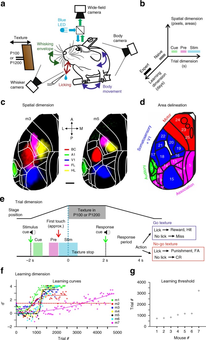
Fig. 1
Spatiotemporal dimensions relevant for texture discrimination learning.
a Behavioral setup. b Schematic of the three relevant dimensions. c Functional maps for two example mice (m3 and m5) obtained by overlaying sensory-evoked activity maps for different sensory stimuli. ...
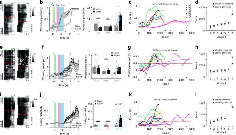
Fig. 2
Motor parameters during theu00a0stim-period are associated with learning.
a Movement probability for go-trials of two example mice plotted as heat maps along the two temporal dimensions (trial dimension on x -axis; learning dimension on y -axis; 50-trial bins along learning...
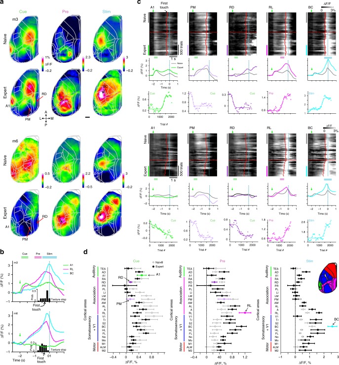
Fig. 3
Changes in wide-field calcium signals across cortex during learning.
a Example activation maps from two mice averaged during cue-, pre-, and stim-period in nau00efve (top) and expert (bottom) phase. Color scale bar indicates min/max of percent u0394 F / F . Overlay of ...
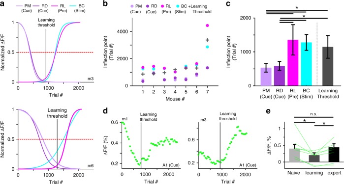
Fig. 4
PM and RD suppression occurs before learning and precedes RL and BC enhancement.
a Normalized sigmoidal fits to the learning-related mean u0394 F / F changes in PM and RD (for cue-period), in RL (for pre-period), and in BC (for stim-period) for two example mice. Horizontal dashed ...
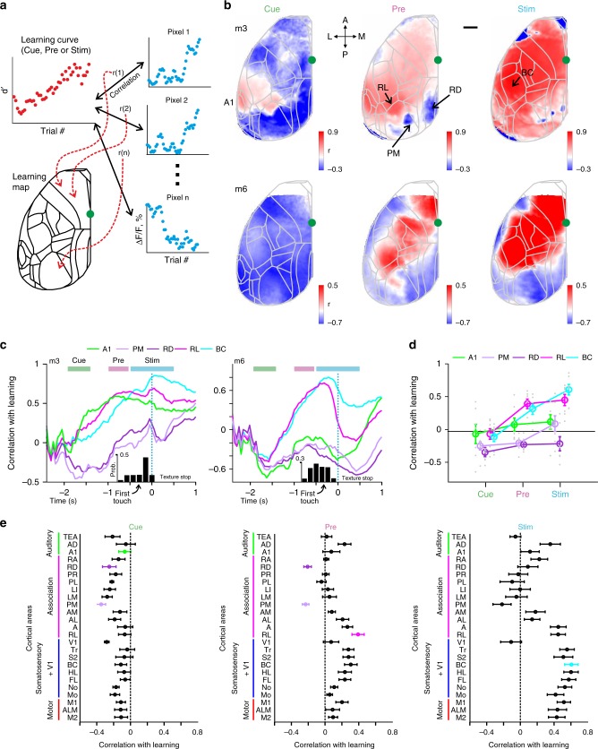
Fig. 5
Learning maps reveal dissociation of association areas in relationship to learning.
a Schematic illustration for calculating a learning map. Each pixel in the maps reflects the correlation coefficient ( r ) between the mouseu2019s learning curve and the curve of learning-related u039...
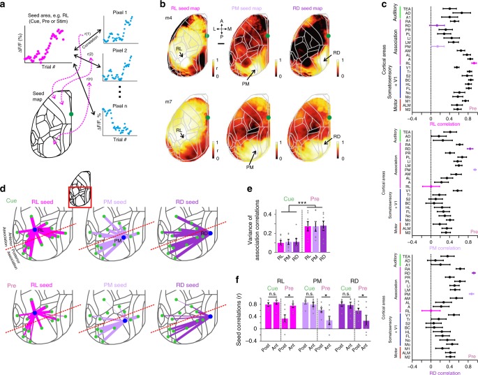
Fig. 6
Functional reorganization of association cortex during learning.
a Schematic of calculating a seed correlation map. Each pixel in the map reflects the correlation coefficient ( r ) between the learning-related u0394 F / F curve of a seed area (e.g. RL, PM, or RD) a...
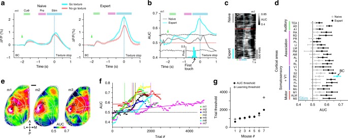
Fig. 7
Emergence of discrimination power in barrel cortex during learning.
a BC activity in an example mouse for go (cyan) and no-go (red) trials in nau00efve (left) and expert (right) mouse. Error bars are s.e.m. across trials. b ROC-AUC values for go vs. no-go trials as a ...
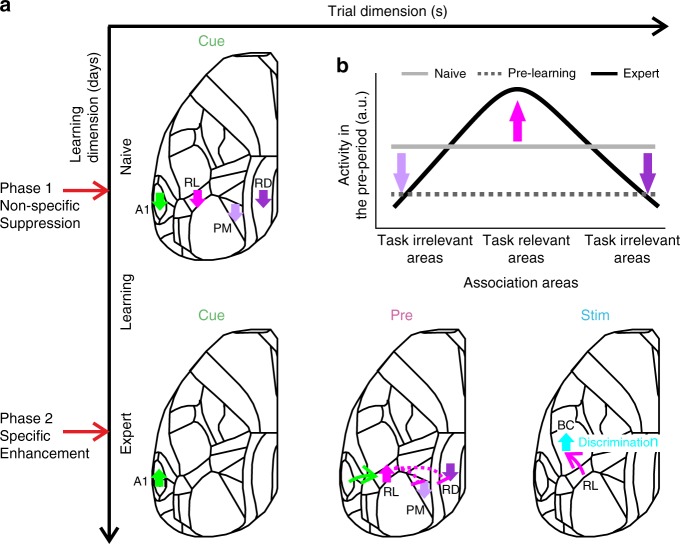
Fig. 8
Learning starts with a general suppression phase followed by a specific enhancement phase.
a A schematic illustration of the main cortical changes withu00a0regard to the two temporal scales: trial ( x -axis) and learning ( y -axis). Two phases occur across learning: before mice actually lea...
Figure images are served from the NIH/NLM PubMed Central Open Access Subset or Europe PMC; copyright remains with the publishers and authors.
💬 Discussion
0 commentsNo comments yet. Be the first to start a discussion!
Leave a Comment