Abstract
AbstractFluorescence polarization microscopy images both the intensity and orientation of fluorescent dipoles and plays a vital role in studying molecular structures and dynamics of bio-complexes. However, current techniques remain difficult to resolve the dipole assemblies on subcellular structures and their dynamics in living cells at super-resolution level. Here we report polarized structured illumination microscopy (pSIM), which achieves super-resolution imaging of dipoles by interpreting the dipoles in spatio-angular hyperspace. We demonstrate the application of pSIM on a series of biological filamentous systems, such as cytoskeleton networks and λ-DNA, and report the dynamics of short actin sliding across a myosin-coated surface. Further, pSIM reveals the side-by-side organization of the actin ring structures in the membrane-associated periodic skeleton of hippocampal neurons and images the dipole dynamics of green fluorescent protein-labeled microtubules in live U2OS cells. pSIM applies directly to a large variety of commercial and home-built SIM systems with various imaging modality.
🔬 Techniques
🔭 Microscopes
💻 Software
✨ Fluorophores
🧪 Sample Preparation
🔬 Cell Lines
🏭 Microscope Brands
🧪 Reagent Suppliers
📷 Detectors
🎨 Filters
💻 Software Details
💻 Code & Software
💾 Data Repositories
🏛️ Research Organizations (ROR)
Affiliated research institutions:
📋 Methods
Reconstruction algorithm for pSIM The pSIM imaging process is described by Eq. ( 1 ), whose Fourier transform is: 2 documentclass[12pt]{minimal} usepackage{amsmath} usepackage{wasysym} usepackage{amsfonts} usepackage{amssymb} usepackage{amsbsy} usepackage{mathrsfs} usepackage{upgreek} setlength{oddsidemargin}{-69pt} begin{document}$$tilde D_{theta ,varphi }({mathbf{k}}_{mathbf{r}},k_alpha ) = left[ {tilde S_{mathrm{p}}({mathbf{k}}_{mathbf{r}},k_alpha ) otimes tilde I_{theta ,varphi }({mathbf{k}}_{mathbf{r}}) otimes tilde F_theta (k_alpha )} right] {mathrm{OTF}}({mathbf{k}}_{mathbf{r}},k_alpha ),\ tilde I_{theta ,varphi }({mathbf{k}}_{mathbf{r}}) = displaystylefrac{{pi I_0}}{4}left[ {delta ({mathbf{k}}_{mathbf{r}}) + frac{1}{2}e^{ivarphi }delta ({mathbf{k}}_{mathbf{r}} - {mathbf{k}}_{mathbf{theta }}) + frac{1}{2}e^{ - ivarphi }delta ({mathbf{k}}_{mathbf{r}} + {mathbf{k}}_{mathbf{theta }})} right],\ tilde F_theta (k_alpha ) = displaystylefrac{{pi eta }}{4}left[ {delta left( {k_alpha } right){mathrm{ + }}frac{1}{2}{e}^{ - 2itheta }delta left( {k_alpha - frac{{mathrm{1}}}{pi }} right){mathrm{ + }}frac{1}{2}{e}^{2itheta }delta left( {k_alpha {mathrm{ + }}frac{{mathrm{1}}}{pi }} right)} right].$$end{document} D ~ θ , φ ( k r , k α ) = S ~ p ( k r , k α ) ⊗ Ĩ θ , φ ( k r ) ⊗ F ~ θ ( k α ) OTF ( k r , k α ) , Ĩ θ , φ ( k r ) = π I 0 4 δ ( k r ) + 1 2 e i φ δ ( k r − k θ ) + 1 2 e − i φ δ ( k r + k θ ) , F ~ θ ( k α ) = π η 4 δ k α + 1 2 e − 2 i θ δ k α − 1 π + 1 2 e 2 i θ δ k α + 1 π . Both the spatially structured illumination documentclass[12pt]{minimal} usepackage{amsmath} usepackage{wasysym} usepackage{amsfonts} usepackage{amssymb} usepackage{amsbsy} usepackage{mathrsfs} usepackage{upgreek} setlength{oddsidemargin}{-69pt} begin{document}$$I_{theta ,varphi }({mathbf{r}})$$end{document} I θ , φ ( r ) and angularly structured illumination F θ ( α ) result in a larger observable reciprocal space in the spatial and polarization dimensions. The reconstruction for pSIM takes two steps: a SIM step and a PM step. For the SIM step, three images belonging to the same pattern are used to solve the three frequency components, as in conventional SIM. However, every frequency component is convoluted with a polarization term documentclass[12pt]{minimal} usepackage{amsmath} usepackage{wasysym} usepackage{amsfonts} usepackage{amssymb} usepackage{amsbsy} usepackage{mathrsfs} usepackage{upgreek} setlength{oddsidemargin}{-69pt} begin{document}$$tilde F_theta (k_alpha )$$end{document} F ~ θ ( k α ) , as shown in Eq. ( 3 ): 3 documentclass[12pt]{minimal} usepackage{amsmath} usepackage{wasysym} usepackage{amsfonts} usepackage{amssymb} usepackage{amsbsy} usepackage{mathrsfs} usepackage{upgreek} setlength{oddsidemargin}{-69pt} begin{document}$$left[ begin{array}{l}tilde D_{theta _{i},varphi _{1}}({mathbf{k}}_{mathbf{r}},k_alpha )\ tilde{D}_{theta _{i},varphi _{2}}({mathbf{k}}_{mathbf{r}},k_alpha )\ tilde{D}_{theta _{i},varphi _{3}}({mathbf{k}}_{mathbf{r}},k_alpha )end{array} right] = {mathbf{M}}_{mathrm{SIM}}left[ begin{array}{l}left[ {tilde S_{mathrm{p}}({mathbf{k}}_{mathbf{r}},k_alpha ) otimes tilde F_{theta _{i}}(k_alpha )} right] {mathrm{OTF}}({mathbf{k}}_{mathbf{r}},k_alpha )\ left[ {tilde{S}_{mathrm{p}}({mathbf{k}}_{mathbf{r}} - {mathbf{k}}_{{mathbf{theta }}_i},k_alpha ) otimes tilde F_{theta _{i}}(k_alpha )} right] {mathrm{OTF}}({mathbf{k}}_{mathbf{r}},k_alpha )\ left[ {tilde S_{mathrm{p}}({mathbf{k}}_{mathbf{r}} + {mathbf{k}}_{{mathbf{theta }}_i},k_alpha ) otimes tilde F_{theta _{i}}(k_alpha )} right] {mathrm{OTF}}({mathbf{k}}_{mathbf{r}},k_alpha )end{array} right];;\ {mathbf{M}}_{mathrm{SIM}} = frac{{pi I_0}}{4}left[ {begin{array}{*{20}{c}} 1 & {displaystylefrac{1}{2}e^{ivarphi _1}} & {displaystylefrac{1}{2}e^{ - ivarphi _1}} \ 1 & {displaystylefrac{1}{2}e^{ivarphi _2}} & {displaystylefrac{1}{2}e^{ - ivarphi _2}} \ 1 & {displaystylefrac{1}{2}e^{ivarphi _{3}}} & {displaystylefrac{1}{2}e^{ - ivarphi _{3}}} end{array}} right].$$end{document} D ~ θ i , φ 1 ( k r , k α ) D ~ θ i , φ 2 ( k r , k α ) D ~ θ i , φ 3 ( k r , k α ) = M SIM S ~ p ( k r , k α ) ⊗ F ~ θ i ( k α ) OTF ( k r , k α ) S ~ p ( k r − k θ i , k α ) ⊗ F ~ θ i ( k α ) OTF ( k r , k α ) S ~ p ( k r + k θ i , k α ) ⊗ F ~ θ i ( k α ) OTF ( k r , k α ) ; M SIM = π I 0 4 1 1 2 e i φ 1 1 2 e − i φ 1 1 1 2 e i φ 2 1 2 e − i φ 2 1 1 2 e i φ 3 1 2 e − i φ 3 . Then, the PM step follows. From the three original spatial components documentclass[12pt]{minimal} usepackage{amsmath} usepackage{wasysym} usepackage{amsfonts} usepackage{amssymb} usepackage{amsbsy} usepackage{mathrsfs} usepackage{upgreek} setlength{oddsidemargin}{-69pt} begin{document}$$tilde S_{mathrm{p}}({mathbf{k}}_{mathbf{r}},k_alpha ) otimes tilde F_{theta _i}(k_alpha ),;i = 1,2,3$$end{document} S ~ p ( k r , k α ) ⊗ F ~ θ i ( k α ) , i = 1 , 2 , 3 , documentclass[12pt]{minimal} usepackage{amsmath} usepackage{wasysym} usepackage{amsfonts} usepackage{amssymb} usepackage{amsbsy} usepackage{mathrsfs} usepackage{upgreek} setlength{oddsidemargin}{-69pt} begin{document}$$tilde S_{mathrm{p}}({mathbf{k}}_{mathbf{r}},k_alpha )$$end{document} S ~ p ( k r , k α ) , documentclass[12pt]{minimal} usepackage{amsmath} usepackage{wasysym} usepackage{amsfonts} usepackage{amssymb} usepackage{amsbsy} usepackage{mathrsfs} usepackage{upgreek} setlength{oddsidemargin}{-69pt} begin{document}$$tilde S_{mathrm{p}}left( {{mathbf{k}}_{mathbf{r}},k_alpha - frac{{mathrm{1}}}{pi }} right)$$end{document} S ~ p k r , k α − 1 π , and documentclass[12pt]{minimal} usepackage{amsmath} usepackage{wasysym} usepackage{amsfonts} usepackage{amssymb} usepackage{amsbsy} usepackage{mathrsfs} usepackage{upgreek} setlength{oddsidemargin}{-69pt} begin{document}$$tilde S_{mathrm{p}}left( {{mathbf{k}}_{mathbf{r}},k_alpha + frac{{mathrm{1}}}{pi }} right)$$end{document} S ~ p k r , k α + 1 π could be further solved with the PM equation (Eq. ( 4 )). SIM uses three illumination pattern directions, which cover the doubled region in reciprocal space. The three polarization directions are sufficient for extracting the dipole orientations, while PM systems usually use additional excitation polarizations to obtain more robust results. Before the PM step, the images are compensated with the calibration data from the fluorescent beads: 4 documentclass[12pt]{minimal} usepackage{amsmath} usepackage{wasysym} usepackage{amsfonts} usepackage{amssymb} usepackage{amsbsy} usepackage{mathrsfs} usepackage{upgreek} setlength{oddsidemargin}{-69pt} begin{document}$$left[ begin{array}{l}tilde S_{mathrm{p}}({mathbf{k}}_{mathbf{r}},k_alpha ) otimes tilde F_{theta _1}(k_alpha )\ tilde S_{mathrm{p}}({mathbf{k}}_{mathbf{r}},k_alpha ) otimes tilde F_{theta _2}(k_alpha )\ tilde S_{mathrm{p}}({mathbf{k}}_{mathbf{r}},k_alpha ) otimes tilde F_{theta _3}(k_alpha )end{array} right] ;= {mathbf{M}}_{mathrm{PM}}left[ begin{array}{l}tilde S_{mathrm{p}}({mathbf{k}}_{mathbf{r}},k_alpha ) {mathrm{OTF}}({mathbf{k}}_{mathbf{r}},k_alpha )\ tilde S_{mathrm{p}}left({mathbf{k}}_{mathbf{r}},k_alpha - displaystylefrac{{mathrm{1}}}{pi }right) {mathrm{OTF}}({mathbf{k}}_{mathbf{r}},k_alpha )\ tilde S_{mathrm{p}}left({mathbf{k}}_{mathbf{r}},k_alpha + displaystylefrac{{mathrm{1}}}{pi }right) {mathrm{OTF}}({mathbf{k}}_{mathbf{r}},k_alpha )end{array} right];;\ {mathbf{M}}_{mathrm{PM}} = frac{{pi eta }}{4}left[ {begin{array}{*{20}{c}} 1 & {displaystylefrac{1}{2}e^{ - 2itheta _1}} & {displaystylefrac{1}{2}e^{2itheta _1}} \ 1 & {displaystylefrac{1}{2}e^{ - 2itheta _2}} & {displaystylefrac{1}{2}e^{2itheta _2}} \ 1 & {displaystylefrac{1}{2}e^{ - 2itheta _3}} & {displaystylefrac{1}{2}e^{2itheta _3}} end{array}} right].$$end{document} S ~ p ( k r , k α ) ⊗ F ~ θ 1 ( k α ) S ~ p ( k r , k α ) ⊗ F ~ θ 2 ( k α ) S ~ p ( k r , k α ) ⊗ F ~ θ 3 ( k α ) ; = M PM S ~ p ( k r , k α ) OTF ( k r , k α ) S ~ p k r , k α − 1 π OTF ( k r , k α ) S ~ p k r , k α + 1 π OTF ( k r , k α ) ; M PM = π η 4 1 1 2 e − 2 i θ 1 1 2 e 2 i θ 1 1 1 2 e − 2 i θ 2 1 2 e 2 i θ 2 1 1 2 e − 2 i θ 3 1 2 e 2 i θ 3 . The three components solved in the PM step, together with the six components documentclass[12pt]{minimal} usepackage{amsmath} usepackage{wasysym} usepackage{amsfonts} usepackage{amssymb} usepackage{amsbsy} usepackage{mathrsfs} usepackage{upgreek} setlength{oddsidemargin}{-69pt} begin{document}$$(tilde S_{mathrm{p}}({mathbf{k}}_{mathbf{r}} pm {mathbf{k}}_{{mathbf{theta }}_i},k_alpha ) otimes tilde F_{theta _i}(k_alpha ),i = 1,2,3)$$end{document} ( S ~ p ( k r ± k θ i , k α ) ⊗ F ~ θ i ( k α ) , i = 1 , 2 , 3 ) solved in the SIM step make up the observable region in the reciprocal space of pSIM (Fig. 1g ). The six high-order spatial components documentclass[12pt]{minimal} usepackage{amsmath} usepackage{wasysym} usepackage{amsfonts} usepackage{amssymb} usepackage{amsbsy} usepackage{mathrsfs} usepackage{upgreek} setlength{oddsidemargin}{-69pt} begin{document}$$(tilde S_{mathrm{p}}({mathbf{k}}_{mathbf{r}} pm {mathbf{k}}_{{mathbf{theta }}_i},k_alpha ) otimes tilde F_{theta _i}(k_alpha ),i = 1,2,3)$$end{document} ( S ~ p ( k r ± k θ i , k α ) ⊗ F ~ θ i ( k α ) , i = 1 , 2 , 3 ) could not be further solved to obtain the separated polarization components documentclass[12pt]{minimal} usepackage{amsmath} usepackage{wasysym} usepackage{amsfonts} usepackage{amssymb} usepackage{amsbsy} usepackage{mathrsfs} usepackage{upgreek} setlength{oddsidemargin}{-69pt} begin{document}$$tilde S_{mathrm{p}}({mathbf{k}}_{mathbf{r}} pm {mathbf{k}}_{{mathbf{theta }}_i},k_alpha )$$end{document} S ~ p ( k r ± k θ i , k α ) and documentclass[12pt]{minimal} usepackage{amsmath} usepackage{wasysym} usepackage{amsfonts} usepackage{amssymb} usepackage{amsbsy} usepackage{mathrsfs} usepackage{upgreek} setlength{oddsidemargin}{-69pt} begin{document}$$tilde S_{mathrm{p}}left( {{mathbf{k}}_{mathbf{r}} pm {mathbf{k}}_{{mathbf{theta }}_i},k_alpha pm frac{{mathrm{1}}}{pi }} right),i = 1,2,3$$end{document} S ~ p k r ± k θ i , k α ± 1 π , i = 1 , 2 , 3 (cross and first harmonics of the frequency components). The nine shifted components are assembled in reciprocal space and an inverse Fourier transform is applied on the spatial dimensions. For PM and pSIM, the polarization response of each pixel is fit to the equation documentclass[12pt]{minimal} usepackage{amsmath} usepackage{wasysym} usepackage{amsfonts} usepackage{amssymb} usepackage{amsbsy} usepackage{mathrsfs} usepackage{upgreek} setlength{oddsidemargin}{-69pt} begin{document}$$I = Acos (2(theta - alpha )) + B$$end{document} I = A cos ( 2 ( θ − α ) ) + B , with θ denoting the polarization and I denoting the image intensity. We use A + B as the intensity signal and α as the dipole orientation. We define documentclass[12pt]{minimal} usepackage{amsmath} usepackage{wasysym} usepackage{amsfonts} usepackage{amssymb} usepackage{amsbsy} usepackage{mathrsfs} usepackage{upgreek} setlength{oddsidemargin}{-69pt} begin{document}$$frac{{{mathrm{2}}A}}{{A + B}}$$end{document} 2 A A + B as the polarization factor, which is equal to the definition reported elsewhere 21 . The detailed derivation of the pSIM algorithm is in Supplementary Note 2 . Unfortunately, the spatio-angular cross harmonics (marked in gray) are unsolvable with the SIM dataset because the excitation polarization θ and the illumination vector k θ are dependent on each other. However, the missing harmonics do not influence either the spatial image or dipole orientation image according to our simulation (Supplementary Fig. 2 ). Our pSIM reconstruction algorithm is based on the previous work of fairSIM ( https://www.fairsim.org/ ) 41 , which is an ImageJ plugin written in Java. However, our data were analyzed by a custom-written MATLAB program for easier debugging. To help the scientific community, we have released our source code on Github ( https://github.com/chenxy2012/PSIM ).
Show full methods section
Reconstruction algorithm for pSIM The pSIM imaging process is described by Eq. ( 1 ), whose Fourier transform is: 2 documentclass[12pt]{minimal} usepackage{amsmath} usepackage{wasysym} usepackage{amsfonts} usepackage{amssymb} usepackage{amsbsy} usepackage{mathrsfs} usepackage{upgreek} setlength{oddsidemargin}{-69pt} begin{document}$$tilde D_{theta ,varphi }({mathbf{k}}_{mathbf{r}},k_alpha ) = left[ {tilde S_{mathrm{p}}({mathbf{k}}_{mathbf{r}},k_alpha ) otimes tilde I_{theta ,varphi }({mathbf{k}}_{mathbf{r}}) otimes tilde F_theta (k_alpha )} right] {mathrm{OTF}}({mathbf{k}}_{mathbf{r}},k_alpha ),\ tilde I_{theta ,varphi }({mathbf{k}}_{mathbf{r}}) = displaystylefrac{{pi I_0}}{4}left[ {delta ({mathbf{k}}_{mathbf{r}}) + frac{1}{2}e^{ivarphi }delta ({mathbf{k}}_{mathbf{r}} - {mathbf{k}}_{mathbf{theta }}) + frac{1}{2}e^{ - ivarphi }delta ({mathbf{k}}_{mathbf{r}} + {mathbf{k}}_{mathbf{theta }})} right],\ tilde F_theta (k_alpha ) = displaystylefrac{{pi eta }}{4}left[ {delta left( {k_alpha } right){mathrm{ + }}frac{1}{2}{e}^{ - 2itheta }delta left( {k_alpha - frac{{mathrm{1}}}{pi }} right){mathrm{ + }}frac{1}{2}{e}^{2itheta }delta left( {k_alpha {mathrm{ + }}frac{{mathrm{1}}}{pi }} right)} right].$$end{document} D ~ θ , φ ( k r , k α ) = S ~ p ( k r , k α ) ⊗ Ĩ θ , φ ( k r ) ⊗ F ~ θ ( k α ) OTF ( k r , k α ) , Ĩ θ , φ ( k r ) = π I 0 4 δ ( k r ) + 1 2 e i φ δ ( k r − k θ ) + 1 2 e − i φ δ ( k r + k θ ) , F ~ θ ( k α ) = π η 4 δ k α + 1 2 e − 2 i θ δ k α − 1 π + 1 2 e 2 i θ δ k α + 1 π . Both the spatially structured illumination documentclass[12pt]{minimal} usepackage{amsmath} usepackage{wasysym} usepackage{amsfonts} usepackage{amssymb} usepackage{amsbsy} usepackage{mathrsfs} usepackage{upgreek} setlength{oddsidemargin}{-69pt} begin{document}$$I_{theta ,varphi }({mathbf{r}})$$end{document} I θ , φ ( r ) and angularly structured illumination F θ ( α ) result in a larger observable reciprocal space in the spatial and polarization dimensions. The reconstruction for pSIM takes two steps: a SIM step and a PM step. For the SIM step, three images belonging to the same pattern are used to solve the three frequency components, as in conventional SIM. However, every frequency component is convoluted with a polarization term documentclass[12pt]{minimal} usepackage{amsmath} usepackage{wasysym} usepackage{amsfonts} usepackage{amssymb} usepackage{amsbsy} usepackage{mathrsfs} usepackage{upgreek} setlength{oddsidemargin}{-69pt} begin{document}$$tilde F_theta (k_alpha )$$end{document} F ~ θ ( k α ) , as shown in Eq. ( 3 ): 3 documentclass[12pt]{minimal} usepackage{amsmath} usepackage{wasysym} usepackage{amsfonts} usepackage{amssymb} usepackage{amsbsy} usepackage{mathrsfs} usepackage{upgreek} setlength{oddsidemargin}{-69pt} begin{document}$$left[ begin{array}{l}tilde D_{theta _{i},varphi _{1}}({mathbf{k}}_{mathbf{r}},k_alpha )\ tilde{D}_{theta _{i},varphi _{2}}({mathbf{k}}_{mathbf{r}},k_alpha )\ tilde{D}_{theta _{i},varphi _{3}}({mathbf{k}}_{mathbf{r}},k_alpha )end{array} right] = {mathbf{M}}_{mathrm{SIM}}left[ begin{array}{l}left[ {tilde S_{mathrm{p}}({mathbf{k}}_{mathbf{r}},k_alpha ) otimes tilde F_{theta _{i}}(k_alpha )} right] {mathrm{OTF}}({mathbf{k}}_{mathbf{r}},k_alpha )\ left[ {tilde{S}_{mathrm{p}}({mathbf{k}}_{mathbf{r}} - {mathbf{k}}_{{mathbf{theta }}_i},k_alpha ) otimes tilde F_{theta _{i}}(k_alpha )} right] {mathrm{OTF}}({mathbf{k}}_{mathbf{r}},k_alpha )\ left[ {tilde S_{mathrm{p}}({mathbf{k}}_{mathbf{r}} + {mathbf{k}}_{{mathbf{theta }}_i},k_alpha ) otimes tilde F_{theta _{i}}(k_alpha )} right] {mathrm{OTF}}({mathbf{k}}_{mathbf{r}},k_alpha )end{array} right];;\ {mathbf{M}}_{mathrm{SIM}} = frac{{pi I_0}}{4}left[ {begin{array}{*{20}{c}} 1 & {displaystylefrac{1}{2}e^{ivarphi _1}} & {displaystylefrac{1}{2}e^{ - ivarphi _1}} \ 1 & {displaystylefrac{1}{2}e^{ivarphi _2}} & {displaystylefrac{1}{2}e^{ - ivarphi _2}} \ 1 & {displaystylefrac{1}{2}e^{ivarphi _{3}}} & {displaystylefrac{1}{2}e^{ - ivarphi _{3}}} end{array}} right].$$end{document} D ~ θ i , φ 1 ( k r , k α ) D ~ θ i , φ 2 ( k r , k α ) D ~ θ i , φ 3 ( k r , k α ) = M SIM S ~ p ( k r , k α ) ⊗ F ~ θ i ( k α ) OTF ( k r , k α ) S ~ p ( k r − k θ i , k α ) ⊗ F ~ θ i ( k α ) OTF ( k r , k α ) S ~ p ( k r + k θ i , k α ) ⊗ F ~ θ i ( k α ) OTF ( k r , k α ) ; M SIM = π I 0 4 1 1 2 e i φ 1 1 2 e − i φ 1 1 1 2 e i φ 2 1 2 e − i φ 2 1 1 2 e i φ 3 1 2 e − i φ 3 . Then, the PM step follows. From the three original spatial components documentclass[12pt]{minimal} usepackage{amsmath} usepackage{wasysym} usepackage{amsfonts} usepackage{amssymb} usepackage{amsbsy} usepackage{mathrsfs} usepackage{upgreek} setlength{oddsidemargin}{-69pt} begin{document}$$tilde S_{mathrm{p}}({mathbf{k}}_{mathbf{r}},k_alpha ) otimes tilde F_{theta _i}(k_alpha ),;i = 1,2,3$$end{document} S ~ p ( k r , k α ) ⊗ F ~ θ i ( k α ) , i = 1 , 2 , 3 , documentclass[12pt]{minimal} usepackage{amsmath} usepackage{wasysym} usepackage{amsfonts} usepackage{amssymb} usepackage{amsbsy} usepackage{mathrsfs} usepackage{upgreek} setlength{oddsidemargin}{-69pt} begin{document}$$tilde S_{mathrm{p}}({mathbf{k}}_{mathbf{r}},k_alpha )$$end{document} S ~ p ( k r , k α ) , documentclass[12pt]{minimal} usepackage{amsmath} usepackage{wasysym} usepackage{amsfonts} usepackage{amssymb} usepackage{amsbsy} usepackage{mathrsfs} usepackage{upgreek} setlength{oddsidemargin}{-69pt} begin{document}$$tilde S_{mathrm{p}}left( {{mathbf{k}}_{mathbf{r}},k_alpha - frac{{mathrm{1}}}{pi }} right)$$end{document} S ~ p k r , k α − 1 π , and documentclass[12pt]{minimal} usepackage{amsmath} usepackage{wasysym} usepackage{amsfonts} usepackage{amssymb} usepackage{amsbsy} usepackage{mathrsfs} usepackage{upgreek} setlength{oddsidemargin}{-69pt} begin{document}$$tilde S_{mathrm{p}}left( {{mathbf{k}}_{mathbf{r}},k_alpha + frac{{mathrm{1}}}{pi }} right)$$end{document} S ~ p k r , k α + 1 π could be further solved with the PM equation (Eq. ( 4 )). SIM uses three illumination pattern directions, which cover the doubled region in reciprocal space. The three polarization directions are sufficient for extracting the dipole orientations, while PM systems usually use additional excitation polarizations to obtain more robust results. Before the PM step, the images are compensated with the calibration data from the fluorescent beads: 4 documentclass[12pt]{minimal} usepackage{amsmath} usepackage{wasysym} usepackage{amsfonts} usepackage{amssymb} usepackage{amsbsy} usepackage{mathrsfs} usepackage{upgreek} setlength{oddsidemargin}{-69pt} begin{document}$$left[ begin{array}{l}tilde S_{mathrm{p}}({mathbf{k}}_{mathbf{r}},k_alpha ) otimes tilde F_{theta _1}(k_alpha )\ tilde S_{mathrm{p}}({mathbf{k}}_{mathbf{r}},k_alpha ) otimes tilde F_{theta _2}(k_alpha )\ tilde S_{mathrm{p}}({mathbf{k}}_{mathbf{r}},k_alpha ) otimes tilde F_{theta _3}(k_alpha )end{array} right] ;= {mathbf{M}}_{mathrm{PM}}left[ begin{array}{l}tilde S_{mathrm{p}}({mathbf{k}}_{mathbf{r}},k_alpha ) {mathrm{OTF}}({mathbf{k}}_{mathbf{r}},k_alpha )\ tilde S_{mathrm{p}}left({mathbf{k}}_{mathbf{r}},k_alpha - displaystylefrac{{mathrm{1}}}{pi }right) {mathrm{OTF}}({mathbf{k}}_{mathbf{r}},k_alpha )\ tilde S_{mathrm{p}}left({mathbf{k}}_{mathbf{r}},k_alpha + displaystylefrac{{mathrm{1}}}{pi }right) {mathrm{OTF}}({mathbf{k}}_{mathbf{r}},k_alpha )end{array} right];;\ {mathbf{M}}_{mathrm{PM}} = frac{{pi eta }}{4}left[ {begin{array}{*{20}{c}} 1 & {displaystylefrac{1}{2}e^{ - 2itheta _1}} & {displaystylefrac{1}{2}e^{2itheta _1}} \ 1 & {displaystylefrac{1}{2}e^{ - 2itheta _2}} & {displaystylefrac{1}{2}e^{2itheta _2}} \ 1 & {displaystylefrac{1}{2}e^{ - 2itheta _3}} & {displaystylefrac{1}{2}e^{2itheta _3}} end{array}} right].$$end{document} S ~ p ( k r , k α ) ⊗ F ~ θ 1 ( k α ) S ~ p ( k r , k α ) ⊗ F ~ θ 2 ( k α ) S ~ p ( k r , k α ) ⊗ F ~ θ 3 ( k α ) ; = M PM S ~ p ( k r , k α ) OTF ( k r , k α ) S ~ p k r , k α − 1 π OTF ( k r , k α ) S ~ p k r , k α + 1 π OTF ( k r , k α ) ; M PM = π η 4 1 1 2 e − 2 i θ 1 1 2 e 2 i θ 1 1 1 2 e − 2 i θ 2 1 2 e 2 i θ 2 1 1 2 e − 2 i θ 3 1 2 e 2 i θ 3 . The three components solved in the PM step, together with the six components documentclass[12pt]{minimal} usepackage{amsmath} usepackage{wasysym} usepackage{amsfonts} usepackage{amssymb} usepackage{amsbsy} usepackage{mathrsfs} usepackage{upgreek} setlength{oddsidemargin}{-69pt} begin{document}$$(tilde S_{mathrm{p}}({mathbf{k}}_{mathbf{r}} pm {mathbf{k}}_{{mathbf{theta }}_i},k_alpha ) otimes tilde F_{theta _i}(k_alpha ),i = 1,2,3)$$end{document} ( S ~ p ( k r ± k θ i , k α ) ⊗ F ~ θ i ( k α ) , i = 1 , 2 , 3 ) solved in the SIM step make up the observable region in the reciprocal space of pSIM (Fig. 1g ). The six high-order spatial components documentclass[12pt]{minimal} usepackage{amsmath} usepackage{wasysym} usepackage{amsfonts} usepackage{amssymb} usepackage{amsbsy} usepackage{mathrsfs} usepackage{upgreek} setlength{oddsidemargin}{-69pt} begin{document}$$(tilde S_{mathrm{p}}({mathbf{k}}_{mathbf{r}} pm {mathbf{k}}_{{mathbf{theta }}_i},k_alpha ) otimes tilde F_{theta _i}(k_alpha ),i = 1,2,3)$$end{document} ( S ~ p ( k r ± k θ i , k α ) ⊗ F ~ θ i ( k α ) , i = 1 , 2 , 3 ) could not be further solved to obtain the separated polarization components documentclass[12pt]{minimal} usepackage{amsmath} usepackage{wasysym} usepackage{amsfonts} usepackage{amssymb} usepackage{amsbsy} usepackage{mathrsfs} usepackage{upgreek} setlength{oddsidemargin}{-69pt} begin{document}$$tilde S_{mathrm{p}}({mathbf{k}}_{mathbf{r}} pm {mathbf{k}}_{{mathbf{theta }}_i},k_alpha )$$end{document} S ~ p ( k r ± k θ i , k α ) and documentclass[12pt]{minimal} usepackage{amsmath} usepackage{wasysym} usepackage{amsfonts} usepackage{amssymb} usepackage{amsbsy} usepackage{mathrsfs} usepackage{upgreek} setlength{oddsidemargin}{-69pt} begin{document}$$tilde S_{mathrm{p}}left( {{mathbf{k}}_{mathbf{r}} pm {mathbf{k}}_{{mathbf{theta }}_i},k_alpha pm frac{{mathrm{1}}}{pi }} right),i = 1,2,3$$end{document} S ~ p k r ± k θ i , k α ± 1 π , i = 1 , 2 , 3 (cross and first harmonics of the frequency components). The nine shifted components are assembled in reciprocal space and an inverse Fourier transform is applied on the spatial dimensions. For PM and pSIM, the polarization response of each pixel is fit to the equation documentclass[12pt]{minimal} usepackage{amsmath} usepackage{wasysym} usepackage{amsfonts} usepackage{amssymb} usepackage{amsbsy} usepackage{mathrsfs} usepackage{upgreek} setlength{oddsidemargin}{-69pt} begin{document}$$I = Acos (2(theta - alpha )) + B$$end{document} I = A cos ( 2 ( θ − α ) ) + B , with θ denoting the polarization and I denoting the image intensity. We use A + B as the intensity signal and α as the dipole orientation. We define documentclass[12pt]{minimal} usepackage{amsmath} usepackage{wasysym} usepackage{amsfonts} usepackage{amssymb} usepackage{amsbsy} usepackage{mathrsfs} usepackage{upgreek} setlength{oddsidemargin}{-69pt} begin{document}$$frac{{{mathrm{2}}A}}{{A + B}}$$end{document} 2 A A + B as the polarization factor, which is equal to the definition reported elsewhere 21 . The detailed derivation of the pSIM algorithm is in Supplementary Note 2 . Unfortunately, the spatio-angular cross harmonics (marked in gray) are unsolvable with the SIM dataset because the excitation polarization θ and the illumination vector k θ are dependent on each other. However, the missing harmonics do not influence either the spatial image or dipole orientation image according to our simulation (Supplementary Fig. 2 ). Our pSIM reconstruction algorithm is based on the previous work of fairSIM ( https://www.fairsim.org/ ) 41 , which is an ImageJ plugin written in Java. However, our data were analyzed by a custom-written MATLAB program for easier debugging. To help the scientific community, we have released our source code on Github ( https://github.com/chenxy2012/PSIM ).
Calibration of the illumination nonuniformity
A slide with 100 nm fluorescent beads was prepared at a proper density so that the beads can be separately localized. The beads were imaged by a 2D-SIM sequence at the largest FOV of the system. For each pattern, three images of the three different phases could calculate the WF image (the zeroth spatial harmonic). If the phase difference is designed as 2 π /3, the WF image could easily be obtained by averaging the three images. In each WF image, the beads were localized by QuickPALM ( http://code.google.com/p/quickpalm ) 42 and their position and intensity were exported. Those beads that appeared in all three images at the same position were used to compensate for the illumination nonuniformity among the different patterns. We either used a quantic polynomial function to fit the nonuniformity or moved the beads at a step size of 500 nm to calibrate the entire FOV. Compensation of the intensity nonuniformity was performed before the PM step during pSIM reconstruction based on Eq. ( 5 ). Detailed information is provided in Supplementary Note 3 : 5 documentclass[12pt]{minimal} usepackage{amsmath} usepackage{wasysym} usepackage{amsfonts} usepackage{amssymb} usepackage{amsbsy} usepackage{mathrsfs} usepackage{upgreek} setlength{oddsidemargin}{-69pt} begin{document}$$D = (S cdot {mathrm{Calib}}) otimes {mathrm{PSF}} to D_{mathrm{calib}} = {it{{cal{F}}}}^{ - 1}left{ {left. {{it{{cal{F}}}}left{ {left. D right}/{mathrm{OTF}}} right.} right}/{mathrm{Calib.}}} right.$$end{document} D = ( S ⋅ Calib ) ⊗ PSF → D calib = F − 1 F D ∕ OTF ∕ Calib.
Experimental measurement of the structured illumination
A sample with a uniform single layer of 20 nm fluorescent beads was prepared to measure the spatio-angular structured illumination, which was excited by structured illumination in our home-built SLM-SIM system. A polarizer in front of the detector was rotated from 0° to 180°, and images were captured every 20°. All the images were rotated to the same angle to make the stripes vertical. Afterwards, columns of the images were averaged to form a row as a spatial dimension. The polarization signals were placed in a column to form the angular dimension (Fig. 1d ). Finally, the frequency domain of the structured illumination in spatio-angular hyperspace was acquired by a 2D Fourier transform (Fig. 1f ). Simulations to verify pSIM The spatio-angular cross-harmonic frequency components are unresolvable by pSIM; thus, pSIM uses the nine obtained frequency pedals to generate a dipole orientation image. If all the components are solved separately, 21 frequency pedals are obtained to fill the entire doubled region (Supplementary Fig. 2 ). To study the influence of the missing cross-harmonic frequencies, we simulated radial lines and circles with dipole orientations parallel to their direction. The simulated samples in the x – y – α coordinate plane were discretized with a spatial grid of 20 nm and an angular grid of 12.5°. Then, we applied a Fourier transform to the simulated data and obtained the corresponding frequency pedals. The frequency components beyond the observable area of pSIM (Supplementary Fig. 1a ) or the entire doubled region were neglected (Supplementary Fig. 2b ). Afterwards, an inverse Fourier transform was applied to obtain super-resolution dipole images. We found that the missing frequency components do not influence either the intensity image or dipole orientations. They only influence the polarization ratio of the sample 3 , which describes the variations in the dipole orientations or the wobbling of dipoles in each pixel. Unexpected high-frequency fluctuations appeared in the super-resolution images of the polarization ratio (Supplementary Fig. 2g ). SIM setup and imaging Supplementary Fig. 3 shows the schematic setup of the home-built SLM-SIM. A laser beam (CNI, MGL-FN-561, 200 mW) was expanded with an achromatic beam expander (Thorlabs, GBE10-B). A half-wave plate (Union, WPA2420-450-650) adjusted the polarization before the laser was passed through a polarization beam splitter (Thorlabs, CCM1-PBS251). A ferroelectric liquid crystal SLM (Fourth Dimension Displays, SXGA-3DM-DEV) controlled the angle and phase of the diffraction pattern. Orders except for the ±1 diffraction orders were blocked with a spatial filter (mask). A vortex half-wave plate (Thorlabs, WPV10 L-532) was used to modulate the polarization of the two ±1 order beams parallel to the interference stripes. A dichroic mirror DM1 (Chroma, ZT561rdc), placed perpendicular to DM2, was introduced to compensate for the polarization ellipticity by switching the incident positions of the s-beam and p-beam. A lens pair was used to relay the ±1 order light spots to the back focal plane of the objective (Nikon, CFI Apochromat TIRF ×100 oil, NA 1.49). The fluorescent signals passed through an emission filter (Semrock, FF01-640/20-25) and reached a sCMOS camera (Tuscen, Dhyana 400BSI). pSIM on the commercial OMX-SIM system (DeltaVision OMX SR, GE, USA) used a ×60 1.4 NA oil immersion objective (Olympus, Japan) and AF488 or AF561 filter sets. Standard 2D-SIM or 3D-SIM sequences were performed with an 80 nm pixel size and 125 nm axial step. pSIM on the commercial N-SIM system (Nikon, Japan) used a ×100 1.49 NA oil immersion objective (Apo TIRF, Nikon, Japan). The 2D-SIM was performed with a 65 nm pixel size.
Sample preparation
The specimens of phalloidin-AF488-labeled F-actin in BAPE cells and phalloidin-AF568-labeled actin in mouse kidney sections were commercially available (FluoCells Prepared Slide #1 and FluoCells Prepared Slide #3, Thermo Fisher). The U2OS cells (ATCC HTB-96 cell line) were cultured in Dulbecco’s modified Eagle’s medium (DMEM) and 10% (v/v) fetal bovine serum (FBS) at 37 °C and 5% CO 2 on 0.17 mm coverslips. Primary culture neurons were cultured from the hippocampus of newborn C57 mice. The use of mice was in accordance with the regulations of the Peking University Animal Care and Use Committee. Fetal hippocampal samples were dissected from the brain and digested with 0.25% trypsin (Invitrogen). Digestion was stopped by adding DMEM-F12 (Gibco) with 10% FBS (Gibco), after which the tissue was dispersed by pipette. After 2 min of precipitation, the supernatant was collected and centrifuged at 500 × g for 2 min. Afterwards, the cells were resuspended in DMEM-F12 with 10% FBS, plated on a coverslip coated with poly- d -lysine (Sigma), and incubated in 5% circulating CO 2 . Neurobasal medium (Gibco) containing pen-strep (Invitrogen), B27 (Gibco), and GlutaMAX (Thermo Fisher) was added to the cells after 4 h. Half of the medium was replaced with fresh medium every 3 days. For immunostaining, the cells were washed with PBS and fixed in 4% PFA (Sigma) at room temperature. Then, the cells were permeabilized in 0.1% Triton at 4 °C, after which they were blocked in 5% donkey serum at room temperature. Phalloidin-AF568 (A12380, Invitrogen) was added for 1 h to label the actin filaments. The cells were washed and mounted on regular slides with ProLong Diamond ( P36970 , Invitrogen), unless otherwise indicated. For GFP labeling, the tubulin-GFP plasmid was transfected into U2OS cells under the standard protocol of Lipofectamine 3000 (L3000, Invitrogen). For λ-DNA, microscope coverslips were first coated with a thin layer of poly-methyl methacrylate to stretch DNA onto the coverslips. SYTOX orange nucleic acid stain (5 mM solution in DMSO, Invitrogen) was diluted 1000-fold. Then, 0.3 μL of a stock λ-DNA solution (300 μg/μL, Invitrogen) was dissolved in 968 μL of PBS, and 32 μL of diluted SYTOX orange was added. Then, 5 μL of the mixed solution was divided into nine drops when added to the coverslips. The coverslips were allowed to air-dry for ~1 h and were sealed with Fixogum rubber cement. The in vitro actin-sliding assays were performed using full-length smooth muscle myosin (SmM-FL) and rabbit striated muscle actin 43 . Approximately 20 μL of 0.4 mg/mL SmM-FL in rigor solution [25 mM imidazole hydrochloride (pH 7.5), 25 mM KCl, 5 mM MgCl 2 , and 1 mM EGTA] was introduced into a nitrocellulose-coated flow chamber and incubated on ice for 10 min. After being incubated on ice for 5 min with 20 μL of 1 mg/mL bovine serum albumin (BSA) in rigor solution, the flow chamber was incubated with 20 μL of a phosphorylation buffer (5.5 μM CaM, 1.3 μM myosin light-chain kinase, 0.2 mM CaCl 2 , 5 mM ATP, 1 mM dithiothreitol, and 5 nM unlabeled F-actin in rigor solution) at 25 °C for 10 min. The flow chamber was washed with 20 μL of 1 mg/mL BSA in rigor solution to remove the unbound proteins and then incubated on ice for 5 min with 20 μL of a 5 nM solution of Alexa Fluor 488-phalloidin-labeled F-actin in actin-sliding buffer I (2.5 mg/mL glucose, 2 Units/mL catalase, and 40 U/mL glucose oxidase in rigor solution). The unbound F-actin was washed away with 20 μL of motility buffer I. Before measurements, the cellulose flow chamber was perfused with 20 μL of motility buffer II (0.5% methylcellulose and 5 mM ATP in motility buffer I).
Statistics and reproducibility
All the figures show the representative data from ≥3 representative experiments. The fitting curves in Figs. 2f and 3f were generated using the Gaussian fitting function in MATLAB. The standard deviations of the dipole orientation angles in Figs. 2f and 3f were analyzed with MATLAB. Reporting summary Further information on research design is available in the Nature Research Reporting Summary linked to this article.
Experimental measurement of the structured illumination
A sample with a uniform single layer of 20 nm fluorescent beads was prepared to measure the spatio-angular structured illumination, which was excited by structured illumination in our home-built SLM-SIM system. A polarizer in front of the detector was rotated from 0° to 180°, and images were captured every 20°. All the images were rotated to the same angle to make the stripes vertical. Afterwards, columns of the images were averaged to form a row as a spatial dimension. The polarization signals were placed in a column to form the angular dimension (Fig. 1d ). Finally, the frequency domain of the structured illumination in spatio-angular hyperspace was acquired by a 2D Fourier transform (Fig. 1f ).
Supplementary information Supplementary Information Peer Review File Description of Additional Supplementary Files Supplementary Movie 1 Supplementary Movie 2 Supplementary Movie 3 Supplementary Movie 4 Supplementary Movie 5 Reporting Summary
📊 Figures
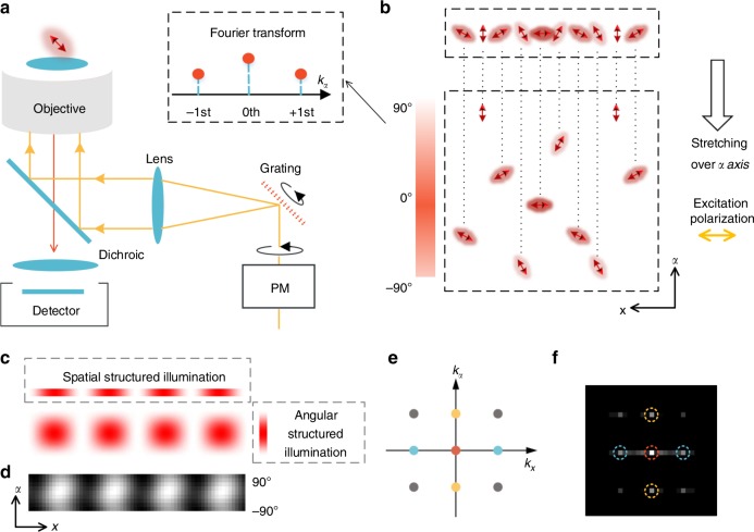
Fig. 1
Principle of polarized structured illumination microscopy (pSIM). a A schematic setup of a typical SIM system. The excitation polarization rotates with the grating to keep the laser beams s-polarized,...
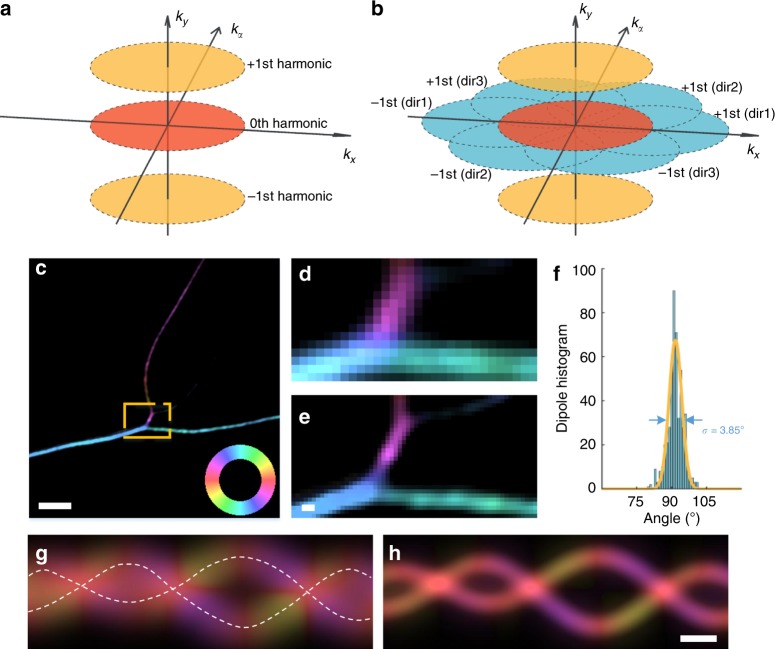
Fig. 2
Comparison between polarization modulation (PM) and pSIM imaging. a The reciprocal space of PM microscopy, including the three harmonics. The zeroth harmonic determines the intensity of the image, whi...
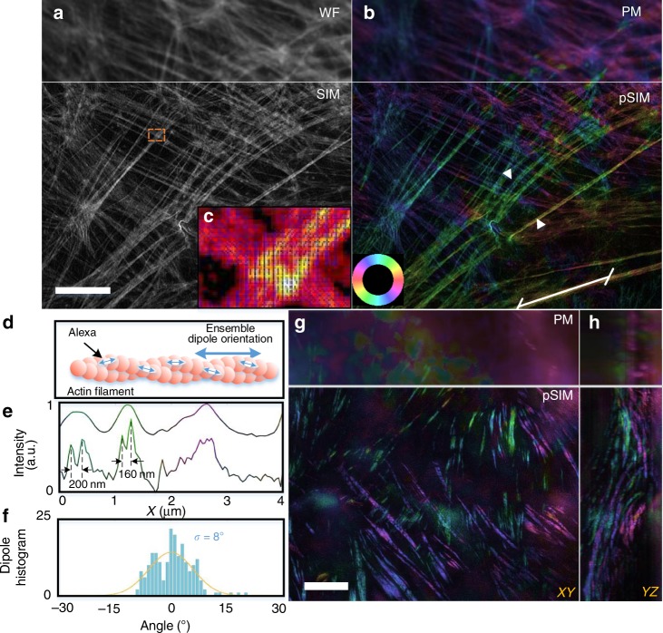
Fig. 3
pSIM imaging results. a , b 2D-SIM and 2D-pSIM images of phalloidin-labeled actin in BAPE cells. a The intensity image in which the upper section is the wide-field (WF) results and the lower section i...
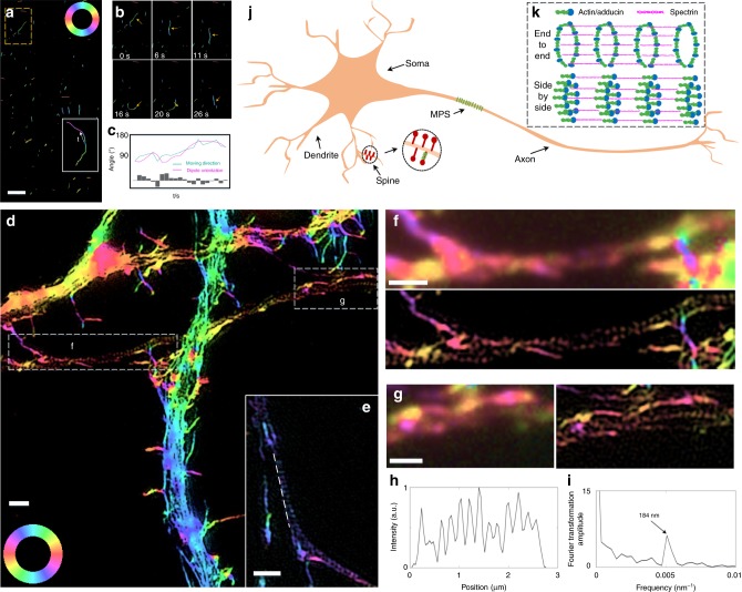
Fig. 4
Imaging the orientation of short actin filaments. a Dynamic imaging of the myosin-driven movement of phalloidin-labeled actin filament. The white box contains the trajectory of a short actin filament....
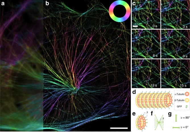
Fig. 5
Live-cell imaging of the microtubules in U2OS cells. a , b 3D-pSIM images, obtained at 0.67 reconstructed fps, of the microtubules in a live U2OS cell (80u2009u00d7u200980u2009u00d7u20090.75u2009u03bc...
Figure images are served from the NIH/NLM PubMed Central Open Access Subset or Europe PMC; copyright remains with the publishers and authors.
💬 Discussion
0 commentsNo comments yet. Be the first to start a discussion!
Leave a Comment