Abstract
Histone modifications influence higher-order chromatin structures at individual epigenomic states and chromatin environments to regulate gene expression. However, genome-wide higher-order chromatin structures shaped by different histone modifications remain poorly characterized. With stochastic optical reconstruction microscopy (STORM), we characterized the higher-order chromatin structures at their epigenomic states, categorized into three major types in interphase: histone acetylation marks form spatially segregated nanoclusters, active histone methylation marks form spatially dispersed larger nanodomains, and repressive histone methylation marks form condensed large aggregates. These distinct structural characteristics are also observed in mitotic chromosomes. Furthermore, active histone marks coincide with less compact chromatin and exhibit a higher degree of co-localization with other active marks and RNA polymerase II (RNAP II), while repressive marks coincide with densely packed chromatin and spatially distant from repressive marks and active RNAP II. Taken together, super-resolution imaging reveals three distinct chromatin structures at various epigenomic states, which may be spatially coordinated to impact transcription.
🔬 Techniques
🔭 Microscopes
🧬 Organisms
💻 Software
✨ Fluorophores
🧪 Sample Preparation
🔬 Cell Lines
🏭 Microscope Brands
🧪 Reagent Suppliers
🔎 Objectives
💻 Software Details
🏛️ Research Organizations (ROR)
Affiliated research institutions:
📋 Methods
Sample Preparation
MCF-10A cells were maintained in DMEM/F12 medium supplemented with 5% horse serum, 10 mg/mL insulin, 20 ng/mL EGF, 0.5 mg/mL hydrocortisone, and 100 ng/mL cholera toxin. MEFs (mouse embryonic fibroblasts) and U2OS (human bone osteosarcoma epithelial) cells were cultured in DMEM supplemented with 10% fetal bovine serum (FBS). Cell line was authenticated by STR DNA Profiling in Genetica DNA Laboratories. Gene loci profiles were verified using DSMZ reference databases. We first coated the glass-bottom dish (World Precision Instruments, FD3510) with 200 μL diluted 100-nm gold nanoparticle solution (1:60 with double-distilled water [ddH 2 O], EM.GC100, BBI Solutions) for 3 hr as the fiducial markers during STORM imaging ( Ma et al., 2017 ). Then, cells were plated onto the dish at an initial confluency of about 50% and cultured overnight to let the cells attach to the dish. To perform immunostaining, the culture medium was aspirated, and the cells were washed with PBS once and fixed in a 1:1 ethanol:methanol solution for 6 min at −20°C. After being washed once with PBS, the cells were blocked by incubation with blocking buffer (3% BSA, 0.05% Triton X-100 in PBS) for 2 hr and were then incubated with one or both primary antibodies diluted in blocking buffer at 4°C overnight. The cells were washed 3 times with washing buffer (0.2% BSA, 0.05% Triton X-100 in PBS) for 5 min per wash, and the corresponding secondary antibodies in the blocking buffer were added to the sample and incubated for 2 hr, protected from light. The cells were washed again three times with washing buffer, washed once with PBS for 5 min, and stored in PBS before imaging. Immediately before imaging, the buffer was switched to the STORM imaging buffer containing 10% (w/v) glucose (Sigma-Aldrich), 0.56 mg/mL glucose oxidase (Sigma-Aldrich), and 0.17 mg/mL catalase (Sigma-Aldrich). For single-color imaging, 0.14 M β-mercaptoethanol (Sigma-Aldrich) was used; for two-color imaging, 0.1 M mercaptoethylamine (MEA) (Sigma-Aldrich) was used. To exclude the potential fixation artifacts, the three most commonly used fixation methods for nuclear staining were evaluated. The STORM images of an active mark, a repressive mark, and active RNAP II from three fixation methods show similar structures of nanoclusters (see also Supplemental Experimental Procedures and Figure S6 ).
Show full methods section
Sample Preparation
MCF-10A cells were maintained in DMEM/F12 medium supplemented with 5% horse serum, 10 mg/mL insulin, 20 ng/mL EGF, 0.5 mg/mL hydrocortisone, and 100 ng/mL cholera toxin. MEFs (mouse embryonic fibroblasts) and U2OS (human bone osteosarcoma epithelial) cells were cultured in DMEM supplemented with 10% fetal bovine serum (FBS). Cell line was authenticated by STR DNA Profiling in Genetica DNA Laboratories. Gene loci profiles were verified using DSMZ reference databases. We first coated the glass-bottom dish (World Precision Instruments, FD3510) with 200 μL diluted 100-nm gold nanoparticle solution (1:60 with double-distilled water [ddH 2 O], EM.GC100, BBI Solutions) for 3 hr as the fiducial markers during STORM imaging ( Ma et al., 2017 ). Then, cells were plated onto the dish at an initial confluency of about 50% and cultured overnight to let the cells attach to the dish. To perform immunostaining, the culture medium was aspirated, and the cells were washed with PBS once and fixed in a 1:1 ethanol:methanol solution for 6 min at −20°C. After being washed once with PBS, the cells were blocked by incubation with blocking buffer (3% BSA, 0.05% Triton X-100 in PBS) for 2 hr and were then incubated with one or both primary antibodies diluted in blocking buffer at 4°C overnight. The cells were washed 3 times with washing buffer (0.2% BSA, 0.05% Triton X-100 in PBS) for 5 min per wash, and the corresponding secondary antibodies in the blocking buffer were added to the sample and incubated for 2 hr, protected from light. The cells were washed again three times with washing buffer, washed once with PBS for 5 min, and stored in PBS before imaging. Immediately before imaging, the buffer was switched to the STORM imaging buffer containing 10% (w/v) glucose (Sigma-Aldrich), 0.56 mg/mL glucose oxidase (Sigma-Aldrich), and 0.17 mg/mL catalase (Sigma-Aldrich). For single-color imaging, 0.14 M β-mercaptoethanol (Sigma-Aldrich) was used; for two-color imaging, 0.1 M mercaptoethylamine (MEA) (Sigma-Aldrich) was used. To exclude the potential fixation artifacts, the three most commonly used fixation methods for nuclear staining were evaluated. The STORM images of an active mark, a repressive mark, and active RNAP II from three fixation methods show similar structures of nanoclusters (see also Supplemental Experimental Procedures and Figure S6 ).
Fluorescence Staining of DNA
DNA was stained by using the Click-iT Plus EdU (5-ethynyl-2′-deoxyuridine) Alexa Fluor 647 Imaging Kit (Thermo Fisher Scientific). The cells were plated onto a glass-bottom dish at an initial confluency of about 50% and cultured overnight to let the cells attach to the dish. Diluted Click-iT EdU reaction buffer in culture medium was added to the dish at a final concentration of 1 μM, and cells were incubated with EdU for 24 hr. After incubation, the media were removed and fixed with 4% paraformaldehyde for 15 min. Cells were washed 3 times with PBS and permeabilized with 0.2% Triton X-100 for 15 min. After washing the cells 3 times with 3% BSA in PBS, Click-iT Plus reaction cocktail was added to detect EdU. The cells were incubated with reaction cocktail for 30 min at room temperature and protected from light. The reaction cocktail was then removed and washed twice with 3% BSA in PBS. For two-color co-staining of DNA and histone marks, after being washed out of the reaction cocktail, cells were incubated with the primary antibody against the histone mark at 4°C overnight. The cells were then washed 3 times with the washing buffer (as described earlier in the Sample Preparation section) for 5 min per wash, and the corresponding Cy3B-conjugated secondary antibodies were added to the sample in blocking buffer and incubated for 2 hr at room temperature, being protected from light. The cells were washed again 3 times with washing buffer and once with PBS for 5 min per wash and stored in PBS before imaging. Click-iT Plus reaction cocktails were prepared per the manufacturer’s instructions as follows: for a total volume of 500 μL, cocktails contain 440 μL 1X Click-iT reaction buffer, 10 μL copper protectant, 1.2 μL Alexa Fluor 647 picolyl azide, and 50 μL reaction buffer additive. All components were provided by the manufacturer’s imaging kits.
Immunofluorescence Staining
All histone proteins were labeled using immunofluorescent staining method. The detailed protocols for immunofluorescent staining have been described in our previous publication ( Xu et al., 2017 ). Alexa Fluor 647 conjugated to the secondary antibodies was used for single-color STORM imaging. For two-color STORM imaging of DNA and histone proteins, DNA was labeled by EdU and detected by Alexa Fluor 647 azide, and the detailed protocol was described in our previous publication ( Ma et al., 2017 ). Histone proteins were immuno-stained by the appropriate primary antibodies and Cy3B-conjugated secondary antibodies, and the detailed protocol was previously described ( Xu et al., 2017 ). For two-color STORM imaging based on dye pairs, secondary antibodies labeled with activator-reporter dye pairs (Alexa Fluor 405-Alexa Fluor 647 and Cy2-Alexa Fluor 647) were used, which were conjugated in our laboratory as previously described ( Xu et al., 2017 ).
Data Acquisition Single-color and two-color
STORM images were acquired using our custom-built system on an Olympus IX71 inverted microscope frame with a 100x, NA-1.4 oil immersion objective (UPLSAPO 100XO; Olympus), with each pixel on the camera corresponding to 130 nm on the sample plane, and fiducial markers were used for 3D drift correction as previously described ( Ma et al., 2017 ). Prior to STORM imaging, the focal plane was adjusted so that the cells exhibit clearest nuclear periphery. For single-color STORM imaging, 40,000 frames were acquired at an exposure time of 20 ms. Two-color imaging was conducted sequentially; 30,000 frames of the Alexa Fluor 647 were acquired at an exposure time of 20 ms for each frame and followed with 30,000 frames of Cy3B at the same exposure time. The reconstruction of the super-resolution image was performed using our custom-written program written in MATLAB 2015 (MathWorks) and described in detail in our previous publication ( Ma et al., 2017 ). The final reconstructed super-resolution image was rendered by accumulating all the valid molecules with a pixel size of 10 nm followed by a Gaussian smoothing filter (σ = 10 nm). To correct the chromatic aberration error across different color channels, a low density of multi-color fluorescence beads (TetraSpeck microspheres, 0.1-μm diameter, blue/green/orange/dark red fluorescence, Fisher Scientific) was used to generate the transform map in this paper ( Sigal et al., 2015 ). The optical resolution of our system was characterized to be ~32 nm (see Figure S7 ). Two-color STORM imaging using dye pairs was acquired with N-STORM (Nikon Instruments), as previously described ( Xu et al., 2017 ). The samples were periodically activated with a sequence of 405-nm, 488-nm laser pulses and then imaged with a 647-nm laser. In each switching cycle, one of the activation lasers was turned on for 1 frame, followed by 3 frames of illumination with the red imaging laser. A total of 40,000 frames, including 10,000 activation frames and 30,000 imaging frames, for each channel were acquired. Imaging frames immediately after an activation pulse were recognized as a controlled activation event, and colors were assigned accordingly. A cross-talk subtraction algorithm was used to subtract the non-specific activation signal ( Bates et al., 2007 ). The STORM imaging thickness is about 300 nm.
Statistical Methods
The mean and SEM were calculated using Microsoft Excel. The statistical comparison between two groups was calculated using the Mann-Whitney U test in GraphPad Prism 7.0, and a two-tailed p value at 95% confidence interval was presented throughout the paper. A p value of less than 0.01 is considered significant.
Calculation of RDF
The calculation of RDF, also known as pair-correlation function, was performed based on an established method written in MATLAB 2015 (MathWorks) ( Caetano et al., 2015 ). In brief, for each cell nucleus, we divided the entire segmented cell nucleus into a maximum possible number of non-overlapping sub-regions with a size of 500 nm × 500 nm. Within each sub-region, we calculated the RDF by adapting the function “spatialStats” in the published software package MIiSR ( Caetano et al., 2015 ). The RDF quantifies the density of localized spots as a function of distance (r) to other localized spots (self-clustering) based on the original coordinates of localized spots (or single molecules) from a single color. It illustrates the presence of multiple cluster sizes and intercluster distance without any assumptions on the shape of the clusters, and the relative degree of clustering is indicated by the height of the peaks corresponding to the molecular clusters ( Caetano et al., 2015 ).
Calculation of Mean Size and SD based on Gaussian Clustering
The details of the Gaussian clustering method have been described in our previous publication ( Ma et al., 2017 ). Figure S7 shows the process of cluster analysis together with the selected parameters. For each cell nucleus, the histogram of the cluster size for each of the histone marks was plotted and fitted with a log-normal distribution ( Figure S8 ). The mean size and SD were calculated by averaging the values from ~20 to 40 nuclei for each histone mark. The histogram ofthe nearest neighbor distances (nnds) ofeach histone mark was shown in Figure S8 .
Calculation of Co-localization
We calculated the DoC (shown in Figures 4 and 5 ) between the histone marks and active RNAP II, based on a published algorithm ( Malkusch et al., 2012 ; Pageon et al., 2016 ), written in MATLAB 2015 (MathWorks). The original coordinates of localized spots (or single molecules) from two colors were used as the basis for our calculation. In brief, for each localized spot from a histone mark, we first calculated the gradient density of the histone mark and RNAP II around this localized spot, based on the number of localized spots from the histone mark and RNAP II within circles of increasing radius (a range of 20 to 500 nm at a step size of 10 nm was used), respectively. This gradient density of the histone mark and RNAP II was normalized by their respective gradient density within the area with the maximum radius and then used to calculate the Spearman correlation. The DoC score ranging from –1 (anti-correlated) to 1 (correlated) with respect to the histone mark was assigned to each localized spot.
Statistical Methods
The mean and SEM were calculated using Microsoft Excel. The statistical comparison between two groups was calculated using the Mann-Whitney U test in GraphPad Prism 7.0, and a two-tailed p value at 95% confidence interval was presented throughout the paper. A p value of less than 0.01 is considered significant.
Supplementary Material 1
📊 Figures
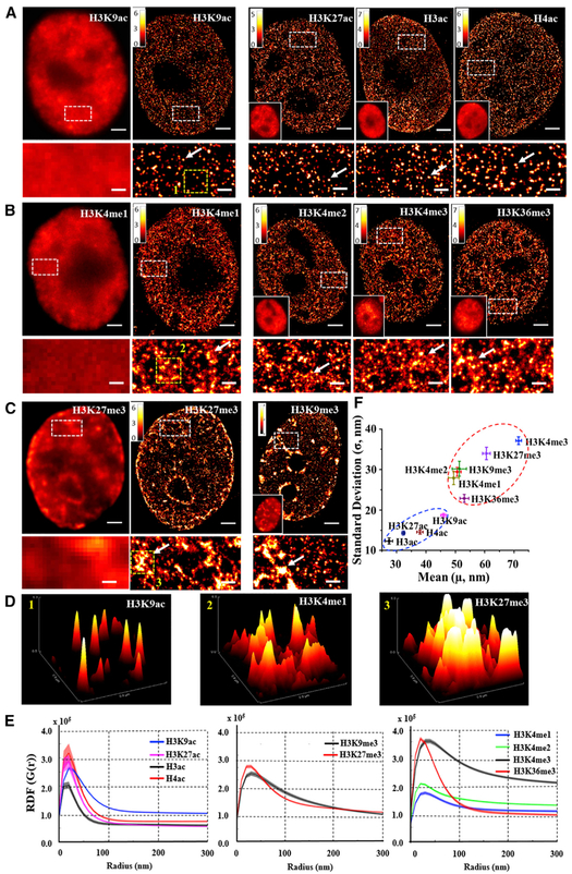
Figure 1.
The STORM Images and Quantitative Characterization of Different Histone Marks
(Au2013C) The representative wide-filed and STORM images of three groups of histone modifications: (A) histone acetylation marks, (B) repressive marks, and (C) active histone methylation marks. The re...
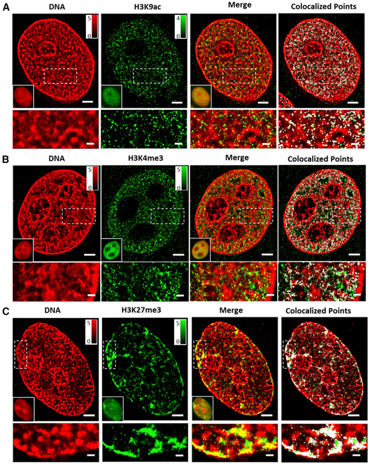
Figure 2.
Two-Color STORM Images of Different Histone Marks and DNA in the Interphase Nuclei
(Au2013C) The representative two-color STORM images showing the spatial relationship between DNA and different histone modifications, ncluding (A) active histone acetylation H3K9ac, (B) active histone...
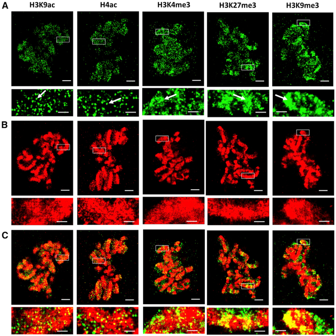
Figure 3.
The Representative Two-Color STORM Images of Different Histone Modification Marks and DNA in the Mitotic Phase
Green channel (A) indicates histone marks (labeled by Cy3B), and red channel (B) indicates DNA (labeled by Alexa Fluor 647). (C) Merged channel. Arrows indicate the presence of the preserved structure...
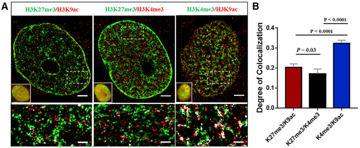
Figure 4.
Two-Color STORM Images of Different Histone Modification Marks
(A) Representative STORM image showing spatial relationship among different histone modifications, categorized into three pairs: active versus repressive histone marks (H3K27me3 versus H3K9ac), bivale...
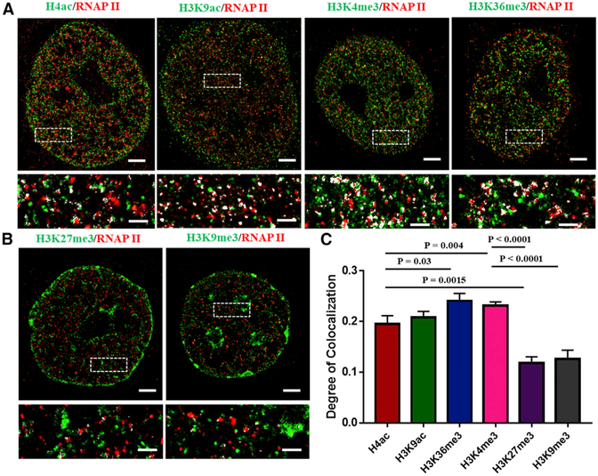
Figure 5.
Representative STORM Images of the Spatial Relationship between Histone Marks and Active RNAP II, or Phosphorylated RNAP II
(A) Active histone marks (H4ac, H3K9ac,H3K4me3, and H3K36me3) versus active RNAP II. (B) Repressive histone marks (H3K27me3, H3K9me3) versus RNAP II. White spots show the co-localized spots. (C) Stati...
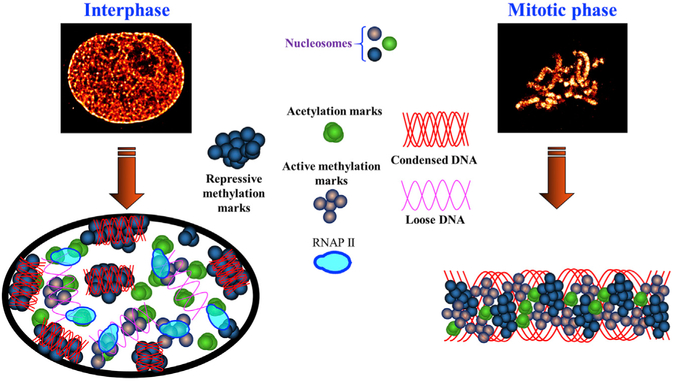
Figure 6.
Model to Depict the Spatial Organization of Chromatin
Model to illustrate the spatial organization of the chromatin environment at interphase and mitotic phase composed of three distinct groups of structural characteristics from active histone acetylatio...
Figure images are served from the NIH/NLM PubMed Central Open Access Subset or Europe PMC; copyright remains with the publishers and authors.
💬 Discussion
0 commentsNo comments yet. Be the first to start a discussion!
Leave a Comment