Abstract
AbstractRecent results from network theory show that complexity affects several dynamical properties of networks that favor synchronization. Here we show that synchronization in 2D and 3D neuronal networks is significantly different. Using dissociated hippocampal neurons we compared properties of cultures grown on a flat 2D substrates with those formed on 3D graphene foam scaffolds. Both 2D and 3D cultures had comparable glia to neuron ratio and the percentage of GABAergic inhibitory neurons. 3D cultures because of their dimension have many connections among distant neurons leading to small-world networks and their characteristic dynamics. After one week, calcium imaging revealed moderately synchronous activity in 2D networks, but the degree of synchrony of 3D networks was higher and had two regimes: a highly synchronized (HS) and a moderately synchronized (MS) regime. The HS regime was never observed in 2D networks. During the MS regime, neuronal assemblies in synchrony changed with time as observed in mammalian brains. After two weeks, the degree of synchrony in 3D networks decreased, as observed in vivo. These results show that dimensionality determines properties of neuronal networks and that several features of brain dynamics are a consequence of its 3D topology.
🔬 Techniques
✨ Fluorophores
🧪 Sample Preparation
🔬 Cell Lines
🏭 Microscope Brands
🧪 Reagent Suppliers
📷 Detectors
🔎 Objectives
🎨 Filters
💻 Software Details
🏛️ Research Organizations (ROR)
Affiliated research institutions:
📋 Methods
Construction of the simulated 3D network and Kuramoto model
In order to construct the 3D network, first we place the nodes (neurons) along a 3D Pythagoras fractal tree. This tree is formed by n = 8 number of iterations, it has a vector scale factor r = [0.5,0.8,0.8] a vector of azimuth angles of the fractal generator phi = [0,2*pi/3,4*pi/3], a vector of polar angles in fractal generator relative to the trunk chi = [pi/3,pi/3,pi/3], and coordinate of the trunk xb, yb and zb given by [0,0],[0,0],[0,1]. This tree can be generated with the FraktalT3D MATLAB code using the command FraktalT3D (n,[0.5,0.8,0.8],[0,2*pi/3,4*pi/3],[pi/3,pi/3,pi/3],[0,0],[0,0],[0,1]). Along the branches of the tree we place randomly the nodes (neurons) of the simulated network with an average density ρ = 3 neurons/unit length. We indicate with N the number of such neurons. The simulated neuronal network is generated by placing short-range links between the neurons i and j with probability and long-range links with probability where d ij is the 3D distance between neuron i and neuron j , and , , δ and α are parameters determining the topology of the network. For a wide range of parameter values the networks generated in this way are small world, have a modular structure and the distribution of the nodes is fractal. On these networks we simulated a Kuramoto model of coupled oscillators, by numerically integrating the equations for i = 1 , 2… N , where θ i is the phase of the oscillator i , K is the parameter determining the intensity of the coupling between the oscillators, ω i is the intrinsic frequency of the oscillator i and is drawn randomly from a Gaussian distribution with zero average and unitary standard deviation, a ij is the adjacency matrix of the network indication which neurons are connected together, and k i is the degree of node i , i.e. In order to evaluate the synchronization property of the 3D network we have measured the order parameter R given by which takes values between 0 and 1. Large values of R indicate phase synchronizations while R ≈ 0 indicates absence of synchronization. We found, that for networks which are at the same time small world and fractal, three different phases of the synchronization dynamics occur as a function of the coupling K . These are: for high values of K , the fully synchronized phase characterized by large values of R which reach a steady state in time, for intermediate values of K , the frustrated synchronization characterized by intermediate values of R which do not reach a steady state in time, and for low values of K , the absence of synchronization characterized by very small values of R . These phases as described in the main text and typical simulations results are shown in Fig. 1e . We note here that the network considered in Fig. 1d,e it is constructed by taking , , α = 2.5 and a dynamics given by equation (3) with K = 1, K = 9 and K = 25 .
Show full methods section
Construction of the simulated 3D network and Kuramoto model
In order to construct the 3D network, first we place the nodes (neurons) along a 3D Pythagoras fractal tree. This tree is formed by n = 8 number of iterations, it has a vector scale factor r = [0.5,0.8,0.8] a vector of azimuth angles of the fractal generator phi = [0,2*pi/3,4*pi/3], a vector of polar angles in fractal generator relative to the trunk chi = [pi/3,pi/3,pi/3], and coordinate of the trunk xb, yb and zb given by [0,0],[0,0],[0,1]. This tree can be generated with the FraktalT3D MATLAB code using the command FraktalT3D (n,[0.5,0.8,0.8],[0,2*pi/3,4*pi/3],[pi/3,pi/3,pi/3],[0,0],[0,0],[0,1]). Along the branches of the tree we place randomly the nodes (neurons) of the simulated network with an average density ρ = 3 neurons/unit length. We indicate with N the number of such neurons. The simulated neuronal network is generated by placing short-range links between the neurons i and j with probability and long-range links with probability where d ij is the 3D distance between neuron i and neuron j , and , , δ and α are parameters determining the topology of the network. For a wide range of parameter values the networks generated in this way are small world, have a modular structure and the distribution of the nodes is fractal. On these networks we simulated a Kuramoto model of coupled oscillators, by numerically integrating the equations for i = 1 , 2… N , where θ i is the phase of the oscillator i , K is the parameter determining the intensity of the coupling between the oscillators, ω i is the intrinsic frequency of the oscillator i and is drawn randomly from a Gaussian distribution with zero average and unitary standard deviation, a ij is the adjacency matrix of the network indication which neurons are connected together, and k i is the degree of node i , i.e. In order to evaluate the synchronization property of the 3D network we have measured the order parameter R given by which takes values between 0 and 1. Large values of R indicate phase synchronizations while R ≈ 0 indicates absence of synchronization. We found, that for networks which are at the same time small world and fractal, three different phases of the synchronization dynamics occur as a function of the coupling K . These are: for high values of K , the fully synchronized phase characterized by large values of R which reach a steady state in time, for intermediate values of K , the frustrated synchronization characterized by intermediate values of R which do not reach a steady state in time, and for low values of K , the absence of synchronization characterized by very small values of R . These phases as described in the main text and typical simulations results are shown in Fig. 1e . We note here that the network considered in Fig. 1d,e it is constructed by taking , , α = 2.5 and a dynamics given by equation (3) with K = 1, K = 9 and K = 25 .
Scaffold preparation
Graphene samples were synthesized using the chemical vapour deposition (CVD) method as described previously 14 49 50 . Briefly, the 3D-GFs were made via CVD using Ni foam as a template, whereas the 2D graphene films were prepared using a Cu foil as substrate. All heavy metal components were then chemically removed, and the substrates were rinsed with HNO 3 , HCl and running water for at least 72 h to remove the etching agents. For sterilization, the scaffolds were treated with UV light for 20 min, followed by decreasing concentrations of ethanol (100%, 75%, 50% for 10 min). Finally, the scaffolds were rinsed with sterile deionized water (twice for 10 min).
Neuronal preparation and culture
Hippocampal neurons from Wistar rats (P2-P3) were prepared in accordance with the guidelines of the Italian Animal Welfare Act, and their use was approved by the Local Veterinary Service, the SISSA Ethics Committee board and the National Ministry of Health (Permit Number: 630-III/14) in accordance with the European Union guidelines for animal care (d.1.116/92; 86/609/C.E.). The animals were anaesthetized with CO 2 and sacrificed by decapitation, and all efforts were made to minimize suffering. All substrates (2D glass coverslips, 2D graphene films and 3D-GFs) were coated with 50 μg/ml poly-L-ornithine (Sigma-Aldrich, St. Louis, MO, USA) overnight, soaked in culture medium overnight and coated with Matrigel just before cells seeding (Corning, Tewksbury MA, USA). Dissociated cells were plated at a concentration of 6 × 10 5 cells/ml on 2D substrates and 2.4 × 10 6 cells/ml on 3D-GF in minimum essential medium (MEM) with GlutaMAX TM supplemented with 10% foetal bovine serum (FBS, all from Invitrogen, Life Technologies, Gaithersburg, MD, USA), 0.6% D-glucose, 15 mM Hepes, 0.1 mg/ml apo-transferrin, 30 μg/ml insulin, 0.1 μg/ml D-biotin, 1 μM vitamin B12 (all from Sigma-Aldrich), and 2.5 μg/ml gentamycin (Life Technologies). After 48 hours, 2 μM cytosine-β - D-arabinofuranoside (Ara-C; Sigma-Aldrich) was added to the culture medium to block glial cell proliferation, and the concentration of FBS was decreased to 5%. Half of the medium was changed every 2–3 days. The neuronal cultures were maintained in an incubator at 37 °C, 5% CO 2 and 95% relative humidity. The cell concentration was adjusted to ensure comparable cell numbers on all substrates. Unlike the 2D substrates, on which all plated cells uniformly deposit on the surface, the 3D-GFs retain cells, which permeate the pores.
Calcium Imaging
The cells were loaded with a cell-permeable calcium dye Fluo4-AM (Life Technologies) by incubating them with 4 μM Fluo4-AM (dissolved in anhydrous DMSO (Sigma-Aldrich), stock solution 4 mM) and Pluronic F-127 20% solution in DMSO (Life Technologies) at a ratio of 1:1 in Ringer’s solution (145 mM NaCl, 3 mM KCl, 1.5 mM CaCl 2 , 1 mM MgCl 2 , 10 mM glucose and 10 mM Hepes, pH 7.4) at 37 °C for 1 hour. After incubation, the cultures were washed and then transferred to the stage of a Nikon Eclipse Ti-U inverted microscope equipped with a piezoelectric table (Nano-ZI Series 500 μm range, Mad City Labs), an HBO 103 W/2 mercury short arc lamp (Osram, Munich, Germany), a mirror unit (exciter filter BP 465–495 nm, dichroic 505 nm, emission filter BP 515–555) and an Electron Multiplier CCD Camera C9100-13 (Hamamatsu Photonics, Japan). The experiments were performed at RT, and images were acquired using the NIS Element software (Nikon, Japan) with an S-Fluor 20x/0.75 NA objective at a sampling rate of 3–10 Hz with a spatial resolution of 256 × 256 pixels for 10–20 min. To avoid saturation of the signals, excitation light intensity was attenuated by ND4 and ND8 neutral density filters (Nikon). Data Analysis Ca 2+ imaging processing and analysis The initial video was processed with the ImageJ (U. S. National Institutes of Health, Bethesda, MA) software. The image sequences were then analysed as described previously 51 . Briefly, neurons were localized, and an appropriate region of interest (ROI) was selected to subtract the background. Appropriate ROIs around the cells bodies were then selected. The time course of the fluorescence intensity, I f (t), in this ROI was displayed, and any decay, which is a consequence of dye bleaching, was evaluated. The Ca 2+ transients of each cell signal were extracted in a semi-automatic manner by selecting a threshold for the smallest detectable peak that was equal to three times the standard deviation of the baseline. Subsequently, the decay of I f (t) was fitted to a cubic spline interpolating I f (t) at 10 or 20 points. I f (t) was then fitted to the original optical signal to compensate for dye bleaching, and the fractional optical signal was calculated as follows: DF/F = (Y(t)+I f (t))/I f (0), where I f (0) is the fluorescence intensity at the beginning of the recording. Computation of raster plot and correlation coefficient of Ca 2+ transient occurrence The times, t i , at which transient peaks occurred are presented in a conventional raster plot. To isolate the smaller transients from the larger ones, the single traces were considered independently. The amplitude distribution of peaks was calculated to separate the two different classes of events. Based on this distribution, a threshold was set to approximately 30% of the maximum amplitude. All peaks under the threshold were considered small, whereas all other peaks were considered to be large calcium transients. The correlation coefficient of the calcium transients for neuron i and neuron j ( σ CTij ) was computed as follows: The total recording time, T tot , was divided into N intervals (1,..,n,…,N) of a duration Δt . Thus, if f in and f jn are the number of calcium transients of neuron i and neuron j in the time interval Δt n , then such that σ CTij depends on Δt and varies between 0 and 1. The range of explored values of Δt was 20 s. Computation of cross-correlation of slow Ca 2+ oscillation Because we observed that Ca 2+ transients can occur both during a positive phase and a negative phase of Ca 2+ fluctuation, we also analysed and computed the correlation coefficient of slow Ca 2+ oscillation. The correlation coefficient of this type of oscillation can be negative, whereas σ CTij can only vary between 0 and 1. The correlation coefficient of slow Ca 2+ oscillation obtained for neuron i and neuron j ( σ SLOWij ) was computed as follows: If s in is the slow signal from neuron i at time t n , its mean value, 〈 s i 〉, is given by where N is the total number of available samples. so that σ SLOWij varies between −1 and 1 and σ SLOWij was computed at the same time interval of σ CTij .
Morphological and immunocytochemical analysis
Cells were fixed in 4% paraformaldehyde containing 0.15% picric acid in phosphate-buffered saline (PBS), saturated with 0.1 M glycine, permeabilized with 0.1% Triton X-100, saturated with 0.5% BSA (all from Sigma-Aldrich) in PBS and then incubated for 1 h with primary antibodies: mouse monoclonal glial fibrillary acidic protein (GFAP), rabbit polyclonal against MAP2 and GABA (all from Sigma-Aldrich), anti-β-tubulin III (TUJ1) and SMI 312 mouse monoclonal antibodies (Covance, Berkeley, CA). The secondary antibodies were goat anti-rabbit Alexa Fluor ® 488, goat anti-mouse Alexa Fluor ® 594, goat anti-mouse immunoglobulin (Ig) G 1 Alexa Fluor ® 488, goat anti-mouse IgG 2a Alexa Fluor ® 594, (all from Life Technologies) and the incubation time was 30 min. Nuclei were stained with 2 μg/ml in PBS Hoechst 33342 (Sigma-Aldrich) for 5 min. All the incubations were performed at room temperature (20–22 °C). The cells were examined using a Leica DM6000 fluorescent microscope equipped with DIC and fluorescence optics, CCD camera and Volocity 5.4 3D imaging software (PerkinElmer, Coventry, UK). The fluorescence images were collected with a 20x magnification and 0.5 NA objective. For each image at least 30 slices were acquired with slice spacing of 0.5 μm. Image J by W. Rasband (developed at the U.S. National Institutes of Health and available at http://rsbweb.nih.gov/ij/ ) was used for image processing.
Statistical analysis
Data are shown as the mean ± s.e.m from at least three neuronal cultures. For the morphological analysis of immunofluorescence images ( Fig. 2 ), n refers to the number of images analysed, and the number in brackets refers to total number of cells analysed. The quantified activity (IEI and Cross-correlation) and morphological data were analysed with the ANOVA test followed by post hoc comparisons using the software SygmaPlot 10.0. Differences among two groups were evaluated with Kolmogorov-Smirnov test, Student’s-t test or Mann-Whitney test (Statistica 6.0 – StatSoft Italy). The number of replicates and statistical tests used for each experiment are mentioned in the respective figure legends or in the Results. Significance was set to *p < 0.05, **p < 0.01 and ***p < 0.001.
📊 Figures
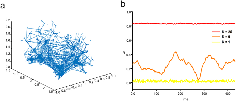
Figure 1
3D network model.
( a ) Simulation of a 3D neuronal network which is modular and has short range connections and some long range connections (small-word network). The neurons are distributed along a fractal tree and pr...
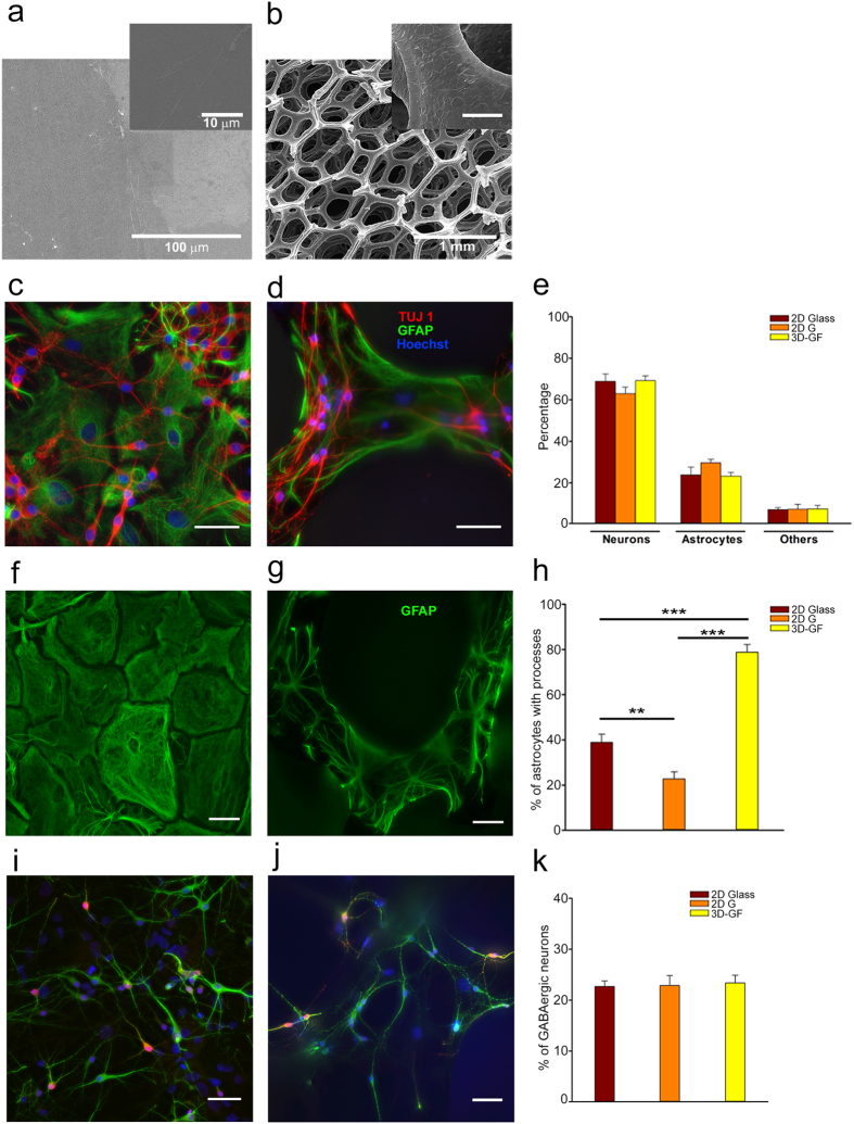
Figure 2
Cellular morphology of 2D and 3D cultures.
( a ) SEM image of a 2D graphene film. Darker areas present an higher number of layers compared to the brighter one; as shown in the inset the surface is flat. ( b ) SEM image of a 3D Graphene Foam sc...
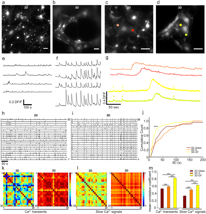
Figure 3
The spontaneous activity of 3D networks is more synchronous.
( a,b ) Neuronal cultures loaded with 4u2009u03bcM Fluo-4-AM calcium indicator on 2D Glass and 3D-GF, respectively. ( c,d ) Glial cells on 2D G and 3D-GF respectively. Coloured circles indicate the RO...
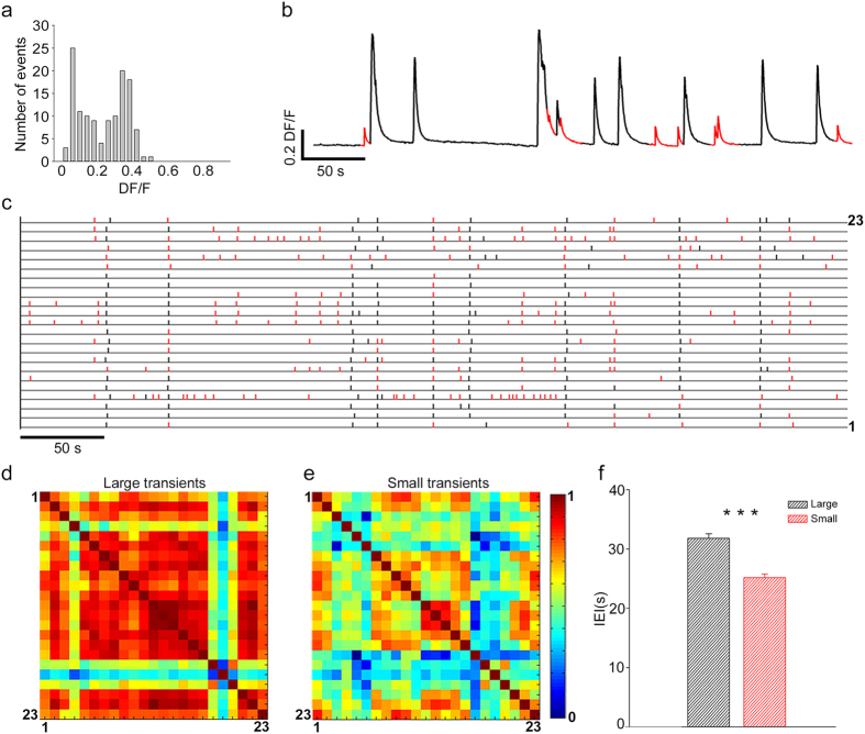
Figure 4
Small and large calcium transients.
( a ) Amplitude histograms of calcium transients obtained from one optical trace: two peaks are clearly present. ( b ) Representative optical trace with large (black) and small (red) calcium transient...
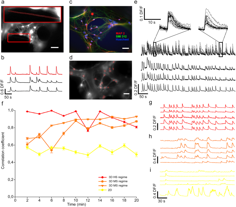
Figure 5
High connectivity leads to HS regime.
( a ) Fluorescent image of a neuronal culture grown on a 3D-GF loaded with Fluo-4 AM; a crossing neurite (inset) and two examples of ROIs (black circles) are shown. ( b ) Optical traces from the cross...
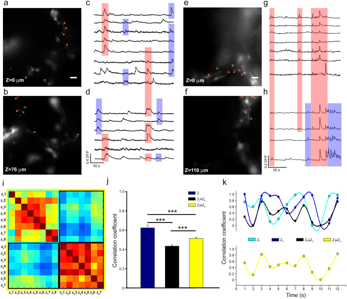
Figure 6
Assemblies of neurons firing in synchrony are dynamic and change both in space and time.
( a,b , e,f ) Fluorescent images of neuronal networks stained by Fluo-4-AM at two focal planes of the same 3D neuronal networks at different z heights (0u201376 and 0u2013110u2009u03bcm respectively)....
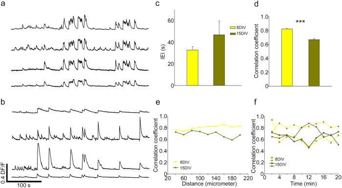
Figure 7
Changes of the degree of correlated activity of 3D neuronal networks during maturation.
( a,b ) Calcium transients of neurons cultured on 3D GF after 8DIV and 15 DIV respectively. ( c ) The mean value of IEI after 8DIV and 15DIV. ( d ) The correlation coefficient shows that there is a re...
Figure images are served from the NIH/NLM PubMed Central Open Access Subset or Europe PMC; copyright remains with the publishers and authors.
💬 Discussion
0 commentsNo comments yet. Be the first to start a discussion!
Leave a Comment