Abstract
AbstractOptical methods capable of manipulating neural activity with cellular resolution and millisecond precision in three dimensions will accelerate the pace of neuroscience research. Existing approaches for targeting individual neurons, however, fall short of these requirements. Here we present a new multiphoton photo-excitation method, termed three-dimensional scanless holographic optogenetics with temporal focusing (3D-SHOT), which allows precise, simultaneous photo-activation of arbitrary sets of neurons anywhere within the addressable volume of a microscope. This technique uses point-cloud holography to place multiple copies of a temporally focused disc matching the dimensions of a neuron’s cell body. Experiments in cultured cells, brain slices, and in living mice demonstrate single-neuron spatial resolution even when optically targeting randomly distributed groups of neurons in 3D. This approach opens new avenues for mapping and manipulating neural circuits, allowing a real-time, cellular resolution interface to the brain.
🔬 Techniques
💻 Software
✨ Fluorophores
🧪 Sample Preparation
🔬 Cell Lines
🏭 Microscope Brands
🧪 Reagent Suppliers
💻 Software Details
🏛️ Research Organizations (ROR)
Affiliated research institutions:
📋 Methods
Ethical statement
All animal experiments were performed in accordance with the guidelines and regulations of the Animal Care and Use Committee of the University of California, Berkeley.
Two-photon absorption characterization
CGH and 3D-SHOT characterization experiments were performed by recording two-photon induced fluorescence on a calibration slide with an inverted microscope. We used a Basler ACa2500 camera, and a Leitz 6.3X Objective to map the entire operational range of the SLM on the camera sensor. We placed two infrared filters along the light-path to eliminate the remaining laser light, leaving only the fluorescence signal in the visible range to be recorded by the camera sensor. For power characterization, we used thick autofluorescent plastic slides (Chroma) to simultaneously collect fluorescence light within the entire volume of excitation from a single focused image. For more precise 3D characterization of two-photon absorption, we used a custom made thin film of fluorescent paint (Tamiya Color TS-36 fluorescent red) sprayed on a microscope glass slide. Here, by mechanically displacing the image acquisition set-up and the photo-excitation pattern (either from CGH or 3D-SHOT), we recorded two-photon absorption in 3D by digitally assembling slice images captured at various depth levels (with micro-metric mechanical increments). The imaging system was calibrated spatially to confirm the effective magnification of the imaging system, and with single target recordings at known power levels to account for non-uniformity in optical transmission across the field of view of the camera. Up to three recordings at various laser power were made to digitally increase the effective dynamic range of the acquisition process. The FWHM was computed first by identifying isolated targets (threshold-based detection) within multi-target holograms, then by computing projections along any axis of interest and by fitting Gaussian profiles to the resulting data.
Show full methods section
Ethical statement
All animal experiments were performed in accordance with the guidelines and regulations of the Animal Care and Use Committee of the University of California, Berkeley.
Two-photon absorption characterization
CGH and 3D-SHOT characterization experiments were performed by recording two-photon induced fluorescence on a calibration slide with an inverted microscope. We used a Basler ACa2500 camera, and a Leitz 6.3X Objective to map the entire operational range of the SLM on the camera sensor. We placed two infrared filters along the light-path to eliminate the remaining laser light, leaving only the fluorescence signal in the visible range to be recorded by the camera sensor. For power characterization, we used thick autofluorescent plastic slides (Chroma) to simultaneously collect fluorescence light within the entire volume of excitation from a single focused image. For more precise 3D characterization of two-photon absorption, we used a custom made thin film of fluorescent paint (Tamiya Color TS-36 fluorescent red) sprayed on a microscope glass slide. Here, by mechanically displacing the image acquisition set-up and the photo-excitation pattern (either from CGH or 3D-SHOT), we recorded two-photon absorption in 3D by digitally assembling slice images captured at various depth levels (with micro-metric mechanical increments). The imaging system was calibrated spatially to confirm the effective magnification of the imaging system, and with single target recordings at known power levels to account for non-uniformity in optical transmission across the field of view of the camera. Up to three recordings at various laser power were made to digitally increase the effective dynamic range of the acquisition process. The FWHM was computed first by identifying isolated targets (threshold-based detection) within multi-target holograms, then by computing projections along any axis of interest and by fitting Gaussian profiles to the resulting data.
Biological samples preparation
The cation channelrhodopsins ChrimsonR and Chronos 52 ; accession: KF992040.1 generated by gene synthesis (Genewiz, South Plainfield, NJ) and anion opsin GtACR1 53 , provided by Dr. John Spudich, University of Texas Health Science Center, Houston) were fused to mRuby2 at the C-terminus at a NotI site (Chronos) or AgeI site (GtACR1) and subcloned into the pCAGGS expression vector between KpnI and XhoI restriction sites by In-Fusion cloning (Clontech, Mountain View, CA). In order to target the opsins to the soma and proximal dendrites of neurons, the sequence encoding the proximal restriction and clustering domain of the Kv2.1 voltage-gated potassium channel consisting of amino acids 536–600 50 , 51 , 54 was codon optimized, synthesized (Integrated DNA Technologies, Coralville, IA) and inserted at the C-terminus of mRuby2 between BsrGI and XhoI restriction sites by In-Fusion cloning. Chinese hamster ovary (CHO) cells were maintained in Ham’s F-12 medium with l -glutamine (Thermo Fisher Scientific, Waltham, MA) containing 10% fetal bovine serum in a humidified incubator at 37 °C and 5% CO 2 . One day prior to transfection, cells were plated on coverglass (Carolina Biological Supply, Burlington, NC) coated with poly-D-lysine (Sigma-Aldrich, St. Louis, MO) so as to reach a confluence of about 80% and transfected with the expression plasmid encoding either Chronos or GtACR1 using Fugene HD (Promega Corporation, Madison, WI) and recorded 24–48 h post transfection. In utero electroporations Electroporations were performed on pregnant CD1 (ICR) mice (E15, Charles River ca. SC:022). For each surgery, the mouse was initially anesthetized with 5% isoflurane and maintained with 2.5% isoflurane. The surgery was conducted on a heating pad, and warm sterile PBS was intermittently perfused over the pups throughout the procedure. A micropipette was used to inject ~2 µl of recombinant DNA at a concentration of 2 µg/µl and into the left ventricle of each neonate’s brain (typically DNA encoding opsins were doped with plasmids expressing GFP or mRuby3 at a concentration of 1:20 to facilitate screening for expression). Fast-green (Sigma-Aldrich) was used to visualize a successful injection. Following successful injection, platinum-plated 5 mm Tweezertrodes (BTX Harvard Apparatus ca. 45-0489) were positioned along the frontal axis across the head of the neonate with the positive electrode of the tweezers positioned against the left side of the head. An Electro Square Porator (BTX Harvard Apparatus ca. 45-0052) was used to administer a train of 5 × 40 mV pulses with a 1 s delay. After the procedure, the mouse was allowed to recover and come to term, and the delivered pups were allowed to develop normally.
Viral infection
Neonatal injections were performed as described 55 . P0-4 EMX1-Cre mice were injected with AAV9-CAG-flexed-ST-ChrimsonR-mRuby2 obtained from the UC Berkeley Vision Science Core Gene Delivery Module. Viral aliquots were loaded into a Drummond Nanoject injector. Neonates were briefly cryo-anesthetized and placed in a head mold. With respect to the lambda suture coordinates for S1 injections were 2.0 mm AP, 3.0 mm L, 0.3 mm DV.
Slice electrophysiology
We used radial slices from the somatosensory barrel cortex cut along the thalamo-cortical plane or coronal cortical sections. The hemisphere was trimmed on both the anterior and posterior side of barrel cortex with coronal cuts, placed on its anterior side and a cut was made with a scalpel so that much of barrel cortex lay in a plane parallel to cut. The surface of this last cut was glued to the slicer tray. The preparation was aided by the use of epifluorescent goggles to visualize the expressing area. Two to three 300–500 µm slices were prepared. Cortical slices (400 µm thick) were prepared 56 from the transfected hemispheres of both male and female mice aged P15−P40 using a DSK Microslicer in a reduced sodium solution containing (in mM) NaCl 83, KCl 2.5, MgSO 4 3.3, NaH 2 PO 4 1, glucose 22, sucrose 72, CaCl 2 0.5, and stored submerged at 34 °C for 30 min, then at room temperature for 1–4 h in the same solution before being transferred to a submerged recording chamber maintained at 30–32 °C by inline heating in a solution containing (in mM) NaCl 119, KCl 2.5, MgSO 4 1.3, NaH 2 PO 4 1.3, glucose 20, NaHCO 3 26, CaCl 2 2.5. CHO cells were recorded in the same media, but with the addition of 5–10 μM all-trans-retinal (Sigma-Aldrich, St. Louis, MO). Recordings were performed in either a Cs + based internal for voltage clamp recordings (CsMeSO 4 135 mM, NaCl 8 mM, HEPES 10 mM, Na 3 GTP 0.3 mM, MgATP 4 mM, EGTA 0.3 mM, QX-314-Cl 5 mM, TEA-Cl 5 mM) or a potassium gluconate based internal for current clamp recordings ( k -gluconate 135 mM, NaCl 8 mM, HEPES 10 mM, Na 3 GTP 0.3 mM, MgATP 4 mM, EGTA 0.3 mM). In most experiments, Alexa Fluor 488 or 594 (Thermo-Fisher) was dissolved into the internal solution to enable morphological recovery. Data were analyzed from recordings in which series resistance remained stable and below 30 MΩ. For measuring photocurrent, cells were included if they had holographic currents > 100 pA; for measurements of action potentials cells were included if holographic stimuli could induce spiking within 200 ms. Data were acquired and filtered at 2.2 kHz using a Multiclamp 700B Amplifier (Axon Instruments) and digitized at 20 kHz (National Instruments). All data were acquired using custom written MATLAB (Mathworks) software. In vivo patch Two-photon guided patch recordings were performed from adult both male and female (35 days or older) wild-type (WT) electroporated adult mice or neonatally injected EMX1-Cre mice (Jackson Labs # 005628). Mice were anesthetized with isofluorane and a custom steel headplate was surgically implanted over the region of interest. A large (2–4 mm diameter) craniotomy was made over the expression site, washed with HEPES ACSF (in mM: NaCl 125, KCl 3, HEPES 10, glucose 10, MgSO 4 ×7 H 2 O 2 , CaCl 2 ×2 H 2 O 2 , set to 300–310 mOsm and pH 7.4) and covered with agarose gel (1%) maintained at 45 °C prior to application. Mice were anesthetized with 1.5 g/kg urethane and 2 µg/kg chlorprothexane before being transferred to recording rig. Body temperature was maintained with a thermal heating pad (FHC) at 37 °C throughout the experiment. Supplementary isofluorane (0–1%) was used to maintain an even level of sedation during recordings, and additional urethane and chlorprothexane was administered every 2–4 h as needed. Cells were identified under a Sutter MOM 2P microscope. Data were acquired using a Multiclamp 700B Amplifier (Axon Instruments) and digitized at 20 kHz (National Instruments). Data was digitally band pass filtered 0.5–2.2 kHz for identification of spikes. All data were acquired using custom written MATLAB (Mathworks) software. Cells were included for analysis if they were spontaneously active and those spikes were sufficiently larger than the noise (>4 Standard deviations of the noise). Furthermore, cells had to pass a 1 P expression check by firing action potentials in response to brief 1 P LED illumination (Lumencore, Sola SE). Cells were holographically stimulated with increasing stimulus durations and laser power until action potentials were reliably generated at 1 Hz stimulation frequency. Spike probability or normalized firing rate was calculated by normalizing the number of action potentials evoked by each stimulus as a function of target position. For in vivo experiments, the minimum number of spikes that occurring during stimulation was subtracted to account for the spontaneous firing rate of the cell. Holographic replication of the CTFP by 3D optical convolution Let documentclass[12pt]{minimal} usepackage{amsmath} usepackage{wasysym} usepackage{amsfonts} usepackage{amssymb} usepackage{amsbsy} usepackage{mathrsfs} usepackage{upgreek} setlength{oddsidemargin}{-69pt} begin{document}$${rm{F}}:Aleft( {x,y} right) to widetilde Aleft( {{k_x},{k_y}} right)$$end{document} F : A x , y → A ~ k x , k y denote the 2D Fourier transform operator, and ( x , y ) the lateral coordinates. The relationship between the CTFP field A C (Supplementary Fig. 1 ), and the field at the input face of the SLM for each component of the spectrum documentclass[12pt]{minimal} usepackage{amsmath} usepackage{wasysym} usepackage{amsfonts} usepackage{amssymb} usepackage{amsbsy} usepackage{mathrsfs} usepackage{upgreek} setlength{oddsidemargin}{-69pt} begin{document}$$Delta k$$end{document} Δ k is given by: 2 documentclass[12pt]{minimal} usepackage{amsmath} usepackage{wasysym} usepackage{amsfonts} usepackage{amssymb} usepackage{amsbsy} usepackage{mathrsfs} usepackage{upgreek} setlength{oddsidemargin}{-69pt} begin{document}$${A_{rm{C}}}left( {x,y,Delta k} right) = {rm{F}}[A_{rm{D}}^ - ]left( {frac{x}{{lambda {f_4}}},frac{y}{{lambda {f_4}}},Delta k} right)$$end{document} A C x , y , Δ k = F [ A D - ] x λ f 4 , y λ f 4 , Δ k We adjusted the phase pattern (focal length of lens L C ) at the diffraction grating so that the dimensions of the beam documentclass[12pt]{minimal} usepackage{amsmath} usepackage{wasysym} usepackage{amsfonts} usepackage{amssymb} usepackage{amsbsy} usepackage{mathrsfs} usepackage{upgreek} setlength{oddsidemargin}{-69pt} begin{document}$$A_{rm{D}}^ -$$end{document} A D - matched the dimensions of the SLM’s short axis to optimize the number of pixels that can be used for holography (Supplementary Fig. 2 ). The SLM applies a phase mask, φ , and the reflected beam becomes: 3 documentclass[12pt]{minimal} usepackage{amsmath} usepackage{wasysym} usepackage{amsfonts} usepackage{amssymb} usepackage{amsbsy} usepackage{mathrsfs} usepackage{upgreek} setlength{oddsidemargin}{-69pt} begin{document}$$A_{rm{D}}^ + left( {x,y,Delta k} right) = A_{rm{D}}^ - left( {x,y,Delta k} right){e^{ivarphi left( {x,y} right)}}$$end{document} A D + x , y , Δ k = A D - x , y , Δ k e i φ x , y Hence: 4 documentclass[12pt]{minimal} usepackage{amsmath} usepackage{wasysym} usepackage{amsfonts} usepackage{amssymb} usepackage{amsbsy} usepackage{mathrsfs} usepackage{upgreek} setlength{oddsidemargin}{-69pt} begin{document}$${rm{F}}left[ {A_{rm{D}}^ + } right] = {rm{F}}left[ {A_{rm{D}}^ - } right] otimes {rm{F}}left[ {{e^{ivarphi }}} right]$$end{document} F A D + = F A D - ⊗ F e i φ where ⊗ represents the 2D convolution product, and F represents the Fourier transform in the ( x , y ) plane. Lens L 5 applies another optical Fourier transform to build the corresponding hologram, which is further demagnified with the tube lens L 6 and the microscope objective L 7 to form the final hologram into the brain. The field A E is given by: 5 documentclass[12pt]{minimal} usepackage{amsmath} usepackage{wasysym} usepackage{amsfonts} usepackage{amssymb} usepackage{amsbsy} usepackage{mathrsfs} usepackage{upgreek} setlength{oddsidemargin}{-69pt} begin{document}$${A_{rm{E}}}left( {x,y,Delta k} right) = {rm{F}}[A_{rm{D}}^ + ]left( {frac{x}{{lambda {f_5}}},frac{y}{{lambda {f_5}}},Delta k} right){e^{ivarphi left( {x,y} right)}}$$end{document} A E x , y , Δ k = F [ A D + ] x λ f 5 , y λ f 5 , Δ k e i φ x , y By combining Equations 2 , 4 , and 5 we find: 6 documentclass[12pt]{minimal} usepackage{amsmath} usepackage{wasysym} usepackage{amsfonts} usepackage{amssymb} usepackage{amsbsy} usepackage{mathrsfs} usepackage{upgreek} setlength{oddsidemargin}{-69pt} begin{document}$${A_{rm{E}}}left( {x,y,Delta k} right) = {A_{rm{C}}}left( {frac{{{f_4}x}}{{{f_5}}},frac{{{f_4}y}}{{{f_5}}},Delta k} right) otimes {rm{F}}[{e^{ivarphi }}]left( {frac{x}{{lambda {f_5}}},frac{y}{{lambda {f_5}}}} right)$$end{document} A E x , y , Δ k = A C f 4 x f 5 , f 4 y f 5 , Δ k ⊗ F [ e i φ ] x λ f 5 , y λ f 5 We deduce the field in 3D by applying Fresnel propagation to each component of the pulse spectrum: 7 documentclass[12pt]{minimal} usepackage{amsmath} usepackage{wasysym} usepackage{amsfonts} usepackage{amssymb} usepackage{amsbsy} usepackage{mathrsfs} usepackage{upgreek} setlength{oddsidemargin}{-69pt} begin{document}$${A_{rm{E}}}left( {x,y,z,Delta k} right) = {A_{rm{E}}}left( {x,y,Delta k} right) otimes hleft( {x,y,z} right)$$end{document} A E x , y , z , Δ k = A E x , y , Δ k ⊗ h x , y , z where documentclass[12pt]{minimal} usepackage{amsmath} usepackage{wasysym} usepackage{amsfonts} usepackage{amssymb} usepackage{amsbsy} usepackage{mathrsfs} usepackage{upgreek} setlength{oddsidemargin}{-69pt} begin{document}$$hleft( {x,y,z} right) = {e^{ikz}}{e^{frac{{ik}}{{2z}}left( {{x^2} + {y^2}} right)}}$$end{document} h x , y , z = e i k z e i k 2 z x 2 + y 2 is the Fresnel propagation kernel. The associativity of the convolution product yields the 3D-SHOT principle where the field to be demagnified and imaged into the sample, documentclass[12pt]{minimal} usepackage{amsmath} usepackage{wasysym} usepackage{amsfonts} usepackage{amssymb} usepackage{amsbsy} usepackage{mathrsfs} usepackage{upgreek} setlength{oddsidemargin}{-69pt} begin{document}$${A_{rm{E}}}left( {x,y,z,Delta k} right)$$end{document} A E x , y , z , Δ k , is a convolution of the CTFP, documentclass[12pt]{minimal} usepackage{amsmath} usepackage{wasysym} usepackage{amsfonts} usepackage{amssymb} usepackage{amsbsy} usepackage{mathrsfs} usepackage{upgreek} setlength{oddsidemargin}{-69pt} begin{document}$${A_{rm{C}}}( {frac{{{f_4}x}}{{{f_5}}},frac{{{f_4}y}}{{{f_5}}},Delta k} )$$end{document} A C ( f 4 x f 5 , f 4 y f 5 , Δ k ) , and the 3D point cloud hologram object, documentclass[12pt]{minimal} usepackage{amsmath} usepackage{wasysym} usepackage{amsfonts} usepackage{amssymb} usepackage{amsbsy} usepackage{mathrsfs} usepackage{upgreek} setlength{oddsidemargin}{-69pt} begin{document}$${rm{F}}[ {{e^{ivarphi }}} ]( {frac{x}{{lambda {f_5}}},frac{y}{{lambda {f_5}}}} ) otimes h( {x,y,z} )$$end{document} F [ e i φ ] ( x λ f 5 , y λ f 5 ) ⊗ h ( x , y , z ) , corresponding to the phase mask, documentclass[12pt]{minimal} usepackage{amsmath} usepackage{wasysym} usepackage{amsfonts} usepackage{amssymb} usepackage{amsbsy} usepackage{mathrsfs} usepackage{upgreek} setlength{oddsidemargin}{-69pt} begin{document}$$varphi ,$$end{document} φ , placed on the SLM. documentclass[12pt]{minimal} usepackage{amsmath} usepackage{wasysym} usepackage{amsfonts} usepackage{amssymb} usepackage{amsbsy} usepackage{mathrsfs} usepackage{upgreek} setlength{oddsidemargin}{-69pt} begin{document}$${A_{rm{E}}}left( {x,y,z,Delta k} right) = {A_{rm{C}}}left( {frac{{{f_4}x}}{{{f_5}}},frac{{{f_4}y}}{{{f_5}}},Delta k} right) otimes left[ {{rm{F}}left[ {{e^{ivarphi }}} right]left( {frac{x}{{lambda {f_5}}},frac{y}{{lambda {f_5}}}} right) otimes hleft( {x,y,z} right)} right]$$end{document} A E x , y , z , Δ k = A C f 4 x f 5 , f 4 y f 5 , Δ k ⊗ F e i φ x λ f 5 , y λ f 5 ⊗ h x , y , z Identification of factors affecting the FWHM by principal component analysis To identify the hologram and brain tissue properties affecting spatial resolution, we used a simple form of principal component analysis (PCA), (Supplementary Notes 7 , 8 ). We consider a diverse data set of multiple holograms for which we gather for each target relevant parameters such as x , y , z location, total number of other targets, brain tissue depth, and distance to the nearest neighbor in a p by k +1 matrix, A, (a last column of ones is used to account for a constant offset). From volume recordings of all the holograms, we record either the radial or axial FWHM in a p by 1 data matrix D. We then compute k +1 by 1 matrix X that minimizes ||D-AX|| 2 . With a diverse enough data set, A×A is invertible and the optimal solution is given by X = (A×A) −1 A×D, The components of X represents the respective contributions of each parameter to the FWHM, with the last one being the constant offset.
Statistics
All statistical analysis was performed with Matlab (Mathworks). The tests performed were Mann−Whitney U -test for two-sample comparisons, Kruskal−Wallis test with multiple comparisons for multiple sample comparison, and F -test of equality of variances. For tests of differences of means, estimates of variance for each group was not typically computed. Each biological replicate is the mean of at least three technical replicates; trial-to-trial variance was extremely low for biological samples. Measurements of fluorescence was performed once per sample. No statistical tests were used to predetermine sample sizes, but we used sample sizes consistent with previous publications 10 , 19 , 45 . Blinding was not used in this study. Unless otherwise noted, all plots with error bars denote mean ± s.e.m. of the indicated number of biological replicates.
Data availability
The data and computer code that support the findings of this study are available from the corresponding author upon reasonable request.
Electronic supplementary material Supplementary Information Peer Review File
📊 Figures
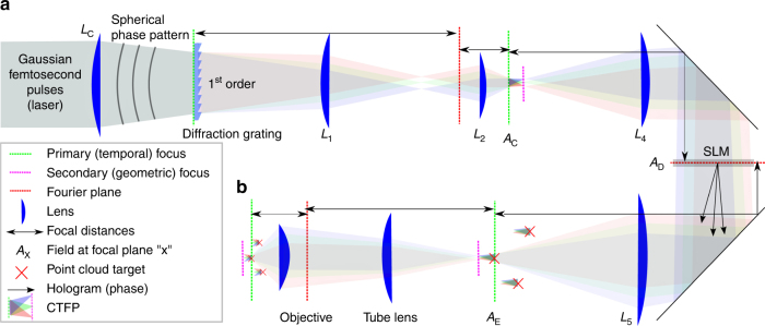
Fig. 1
Simplified experimental set-up for 3D-SHOT. a A spherical phase mask is applied to a Gaussian femtosecond laser pulse incident on a blazed diffraction grating. After the grating, the direction of prop...
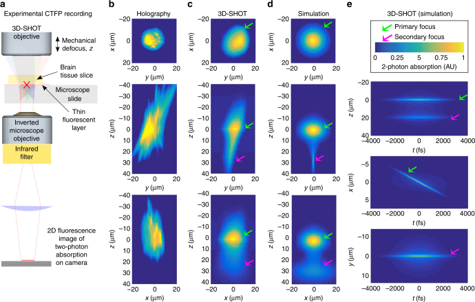
Fig. 2
Optical characterization of the spatial resolution of CGH vs. 3D-SHOT. a We used a fluorescent calibration slide and an inverted microscope to compare two-photon absorption patterns in 3D. b For conve...
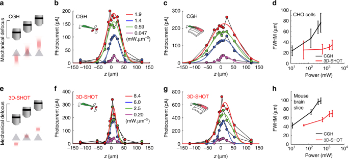
Fig. 3
3D-SHOT generates axially confined photo-activation. a A photostimulation pattern generated with CGH was mechanically stepped along the optical z -axis and passed through a cell expressing opsin. Phot...
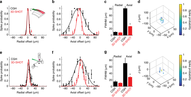
Fig. 4
3D-SHOT provides high spatial resolution photo-activation of neurons in vitro and in vivo. a Spatial profile of two-photon evoked spiking of a L2/3 pyramidal neuron in a mouse brain slice in the radia...
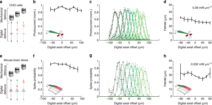
Fig. 5
3D-SHOT provides cellular resolution photostimulation in a large volume through digital focusing. a To quantify the spatial resolution of 3D-SHOT as a function of hologram target depth, we recorded ph...
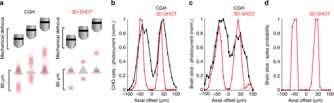
Fig. 6
Single-neuron resolution with simultaneous photostimulation of two targets along the axial dimension. a Using CGH or 3D-SHOT we simultaneously photostimulated two targets separated by 80u2009u00b5m al...
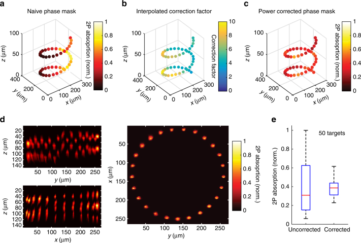
Fig. 7
Power corrected 3D-SHOT simultaneously illuminates 50 spots. a Uncorrected simultaneous 3D-SHOT with a hologram targeting 50 spots in a spiral pattern, occupying 50 individual z- planes. Spots are col...
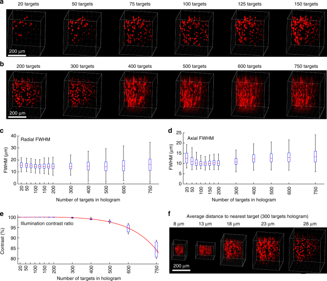
Fig. 8
Spatial resolution with simultaneous targets throughout a large volume. a u2212 b Example 3D renderings from tomographic images of two-photon absorption from single-shot holograms targeting increasing...
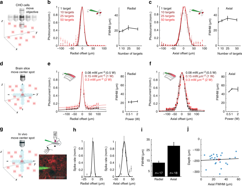
Fig. 9
Spatially precise volumetric optogenetics with 3D-SHOT. a Schematic demonstrating 3D-SHOT stimulation of a CHO cell with a single spot in au00a0hologram targeting multiple spots in the volume. The obj...
Figure images are served from the NIH/NLM PubMed Central Open Access Subset or Europe PMC; copyright remains with the publishers and authors.
💬 Discussion
0 commentsNo comments yet. Be the first to start a discussion!
Leave a Comment