Abstract
Radial spokes (RSs) play an essential role in the regulation of axonemal dynein activity and thus of ciliary and flagellar motility. However, few details are known about the complexes involved. Using cryo-electron tomography and subtomogram averaging, we visualized the three-dimensional structure of the radial spokes in Chlamydomonas flagella in unprecedented detail. Unlike many other species, Chlamydomonas has only two spokes per axonemal repeat, RS1 and RS2. Our data revealed previously uncharacterized features, including two-pronged spoke bases that facilitate docking to the doublet microtubules, and that inner dyneins connect directly to the spokes. Structures of wild type and the headless spoke mutant pf17 were compared to define the morphology and boundaries of the head, including a direct RS1-to-RS2 interaction. Although the overall structures of the spokes are very similar, we also observed some differences, corroborating recent findings about heterogeneity in the docking of RS1 and RS2. In place of a third radial spoke we found an uncharacterized, shorter electron density named "radial spoke 3 stand-in," which structurally bears no resemblance to RS1 and RS2 and is unaltered in the pf17 mutant. These findings demonstrate that radial spokes are heterogeneous in structure and may play functionally distinct roles in axoneme regulation.
🔬 Techniques
🔭 Microscopes
🧬 Organisms
💻 Software
✨ Fluorophores
🧪 Sample Preparation
🏭 Microscope Brands
🧪 Reagent Suppliers
💻 Software Details
🏛️ Research Organizations (ROR)
Affiliated research institutions:
📋 Methods
Axoneme isolation and cryosample preparation All C. reinhardtii strains used in this study are summarized in Table 1 . Cells were grown in liquid Tris-acetate-phosphate medium ( Gorman and Levine, 1965 ) under a 16-h-light/8-h-dark cycle and harvested by 5-min centrifugation at 1100 × g. After two washes, cells were resuspended in a minimal medium containing 10 mM 4-(2-hydroxyethyl)-1-piperazineethanesulfonic acid (HEPES), pH 7.4, 1 mM SrCl 2 , 4% sucrose, and 1 mM dithiothreitol. The pH-shock method ( Witman et al. , 1972 ) was used to detach flagella from cell bodies. After deflagellation, 5 mM MgSO 4 , 1 mM ethylene glycol tetraacetic acid (EGTA), 0.1 mM EDTA, and 100 μg/ml aprotinin, pepstatin, and leupeptin were added to the medium, and cell bodies were pelleted by a 10-min spin at 1800 × g at 4°C. The flagella present in the supernatant were purified in two additional centrifugation steps at 2400 × g and 4°C for 10 min using 5 ml of a 20% sucrose solution as a cushion. The flagellar membrane was removed by detergent treatment for 30 min with 0.1% Nonidet P-40 (Sigma-Aldrich, St. Louis, MO) or 1% IGEPAL CA-630 (Sigma-Aldrich) for 30 min at 4°C. The axonemes were collected by centrifugation at 35,000 × g for 1 h at 4°C. The pelleted axonemes were resuspended in 10 mM HEPES, pH 7.4, 25 mM NaCl, 4 mM MgSO 4 , 1 mM EGTA, and 0.1 mM EDTA and processed within 24 h. Quantifoil holey carbon grids (Quantifoil Micro Tools, Jena, Germany) were glow discharged for 30 s at −40 mA before a drop of a 10-nm colloidal gold solution (Sigma-Aldrich) was applied. After drying, grids were washed by briefly dipping them into Milli-Q purified water (Millipore, Billerica, MA), and excess water was removed with a filter paper (Whatman, Piscataway, NJ). After grids dried completely, they were loaded in a home-made plunge-freezing device ( Trachtenberg, 1993 ), and 3 μl of axoneme sample and 1 μl of a 10-fold-concentrated, 10-nm colloidal gold solution were added to the grid. The mixture was blotted with a filter paper (Whatman #1) from the front side for ∼2 s and immediately plunge frozen in liquid ethane to achieve sample vitrification. Grids were stored in liquid nitrogen until examined by EM. Cryo-ET Details of tilt series acquisition and tomogram reconstruction were published earlier ( Heuser et al. , 2009 ; Nicastro, 2009 ). In brief, cryosamples were transferred into a transmission electron microscope (Tecnai F30; FEI, Hillsboro, OR), which was operated at 300 keV, using a cryoholder (Gatan, Pleasanton, CA). Data acquisition was controlled by the microscope software SerialEM ( Mastronarde, 2005 ). Tilt series were recorded under low-dose conditions by stepwise rotating the sample from −65 to +65° with 1.5–2.5° increments. The cumulative electron dose was limited to ∼100 e/Å 2 . All images were digitally recorded on a 2k × 2k charge-coupled device camera (Gatan) at a magnification of 13,500, resulting in a pixel size of ∼1 nm, at −6 or −8 μm defocus and using an energy filter (Gatan) in zero-loss mode with 20-eV slit width. The IMOD software package ( Kremer et al. , 1996 ) was used for fiducial alignment and cryotomogram reconstruction by weighted backprojection. Only tomograms of noncompressed or mildly compressed and intact axonemes were used for further image processing and data analysis.
Show full methods section
Axoneme isolation and cryosample preparation All C. reinhardtii strains used in this study are summarized in Table 1 . Cells were grown in liquid Tris-acetate-phosphate medium ( Gorman and Levine, 1965 ) under a 16-h-light/8-h-dark cycle and harvested by 5-min centrifugation at 1100 × g. After two washes, cells were resuspended in a minimal medium containing 10 mM 4-(2-hydroxyethyl)-1-piperazineethanesulfonic acid (HEPES), pH 7.4, 1 mM SrCl 2 , 4% sucrose, and 1 mM dithiothreitol. The pH-shock method ( Witman et al. , 1972 ) was used to detach flagella from cell bodies. After deflagellation, 5 mM MgSO 4 , 1 mM ethylene glycol tetraacetic acid (EGTA), 0.1 mM EDTA, and 100 μg/ml aprotinin, pepstatin, and leupeptin were added to the medium, and cell bodies were pelleted by a 10-min spin at 1800 × g at 4°C. The flagella present in the supernatant were purified in two additional centrifugation steps at 2400 × g and 4°C for 10 min using 5 ml of a 20% sucrose solution as a cushion. The flagellar membrane was removed by detergent treatment for 30 min with 0.1% Nonidet P-40 (Sigma-Aldrich, St. Louis, MO) or 1% IGEPAL CA-630 (Sigma-Aldrich) for 30 min at 4°C. The axonemes were collected by centrifugation at 35,000 × g for 1 h at 4°C. The pelleted axonemes were resuspended in 10 mM HEPES, pH 7.4, 25 mM NaCl, 4 mM MgSO 4 , 1 mM EGTA, and 0.1 mM EDTA and processed within 24 h. Quantifoil holey carbon grids (Quantifoil Micro Tools, Jena, Germany) were glow discharged for 30 s at −40 mA before a drop of a 10-nm colloidal gold solution (Sigma-Aldrich) was applied. After drying, grids were washed by briefly dipping them into Milli-Q purified water (Millipore, Billerica, MA), and excess water was removed with a filter paper (Whatman, Piscataway, NJ). After grids dried completely, they were loaded in a home-made plunge-freezing device ( Trachtenberg, 1993 ), and 3 μl of axoneme sample and 1 μl of a 10-fold-concentrated, 10-nm colloidal gold solution were added to the grid. The mixture was blotted with a filter paper (Whatman #1) from the front side for ∼2 s and immediately plunge frozen in liquid ethane to achieve sample vitrification. Grids were stored in liquid nitrogen until examined by EM. Cryo-ET Details of tilt series acquisition and tomogram reconstruction were published earlier ( Heuser et al. , 2009 ; Nicastro, 2009 ). In brief, cryosamples were transferred into a transmission electron microscope (Tecnai F30; FEI, Hillsboro, OR), which was operated at 300 keV, using a cryoholder (Gatan, Pleasanton, CA). Data acquisition was controlled by the microscope software SerialEM ( Mastronarde, 2005 ). Tilt series were recorded under low-dose conditions by stepwise rotating the sample from −65 to +65° with 1.5–2.5° increments. The cumulative electron dose was limited to ∼100 e/Å 2 . All images were digitally recorded on a 2k × 2k charge-coupled device camera (Gatan) at a magnification of 13,500, resulting in a pixel size of ∼1 nm, at −6 or −8 μm defocus and using an energy filter (Gatan) in zero-loss mode with 20-eV slit width. The IMOD software package ( Kremer et al. , 1996 ) was used for fiducial alignment and cryotomogram reconstruction by weighted backprojection. Only tomograms of noncompressed or mildly compressed and intact axonemes were used for further image processing and data analysis.
Image processing
For subtomogram averaging of the 96-nm-long axonemal repeat along the axonemal DMTs we used the program PEET (Particle Estimation for Electron Tomography; Nicastro et al. , 2006 ). The repeats were computationally cut from the raw tomograms, aligned in three dimensions, and averaged with missing wedge compensation, resulting in an average with increased signal-to-noise ratio and improved resolution ( Nicastro et al. , 2006 ; Nicastro, 2009 ). Two different alignment strategies were tested: in the “global alignment” approach the entire 96-nm repeat unit (volume size, 100 × 100 × 80 nm) was used for 3D alignment, whereas the “local alignment” method optimized the alignment for smaller regions (volume sizes were either 90 × 50 × 32 nm centering on RS1, RS2, and RS3S or 66 × 22 × 32 nm centering on the RS head, respectively). For pf17 the global alignment resulted in the best average and is therefore depicted in all figures of pf17 axonemes. In contrast, the local alignment averages resolved the radial spokes at slightly better detail for WT and pWT and are therefore depicted in all figures of WT/pWT except for Figure 3A and Supplemental Figure S1A. Some of the tomograms were previously used, focusing on other axonemal complexes and using different image processing methods ( Heuser et al. , 2009 ; T. Heuser et al. , unpublished results). The resolution of all analyzed strains was estimated at the stem part of RS2 using the Fourier shell correlation method ( Harauz and Van Heel, 1986 ) and the 0.5 criterion ( Table 1 ). The UCSF Chimera software package ( Pettersen et al. , 2004 ) was used to measure volume sizes and to visualize the axonemal averages by isosurface rendering. Masses of RS parts were estimated by assuming an average protein density of 1.43 g/cm 3 ( Quillin and Matthews, 2000 ) and normalizing the isosurface rendering threshold to the mass of DMT ( Heuser et al. , 2009 ). The placement of boundaries between RS1/RS2/RS3S and the IDA tails is based on comparison of our images with single-particle structures of dynein ( Roberts et al. , 2009 ).
📊 Figures
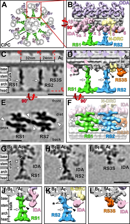
FIGURE 1:
3D structure of RSs in pWT. (A) Composite isosurface rendering of an axoneme cross section viewed from proximal (flagellar base) toward distal (flagellar tip). The CPC is surrounded by nine DMTs, one ...
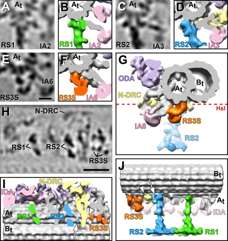
FIGURE 2:
Connections between RSs and neighboring structures. Tomographic slices (A, C, E, H) and isosurface renderings (B, D, F, G, I, J) of the averaged axonemal repeat from pWT show the connections of the ba...
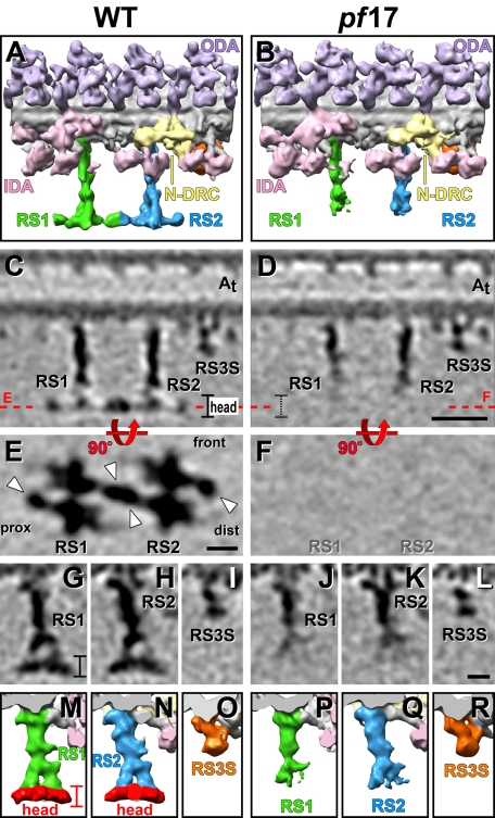
FIGURE 3:
Comparison of the RS structure in WT and the RS-headless mutant pf17. Isosurface renderings (A, B, Mu2013R) and tomographic slices (Cu2013L) from the averaged axonemal repeats of WT and pf17 viewed fr...
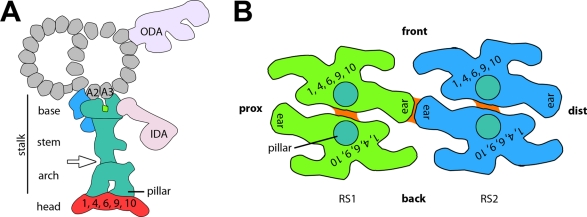
FIGURE 4:
Schematic model of the RS structure in Chlamydomonas flagella. (A) Cross-sectional view from proximal showing, in turquoise, the consensus structure of RSs, that is, the part of the RS that seems cons...
Figure images are served from the NIH/NLM PubMed Central Open Access Subset or Europe PMC; copyright remains with the publishers and authors.
💬 Discussion
0 commentsNo comments yet. Be the first to start a discussion!
Leave a Comment