Abstract
Microtubules polymerize and depolymerize stochastically, a behavior essential for cell division, motility, and differentiation. While many studies advanced our understanding of how microtubule-associated proteins tune microtubule dynamics in trans, we have yet to understand how tubulin genetic diversity regulates microtubule functions. The majority of in vitro dynamics studies are performed with tubulin purified from brain tissue. This preparation is not representative of tubulin found in many cell types. Here we report the 4.2-Å cryo-electron microscopy (cryo-EM) structure and in vitro dynamics parameters of α1B/βI+βIVb microtubules assembled from tubulin purified from a human embryonic kidney cell line with isoform composition characteristic of fibroblasts and many immortalized cell lines. We find that these microtubules grow faster and transition to depolymerization less frequently compared with brain microtubules. Cryo-EM reveals that the dynamic ends of α1B/βI+βIVb microtubules are less tapered and that these tubulin heterodimers display lower curvatures. Interestingly, analysis of EB1 distributions at dynamic ends suggests no differences in GTP cap sizes. Last, we show that the addition of recombinant α1A/βIII tubulin, a neuronal isotype overexpressed in many tumors, proportionally tunes the dynamics of α1B/βI+βIVb microtubules. Our study is an important step toward understanding how tubulin isoform composition tunes microtubule dynamics.
🔬 Techniques
🔭 Microscopes
🧬 Organisms
💻 Software
✨ Fluorophores
🔬 Cell Lines
🏭 Microscope Brands
🧪 Reagent Suppliers
📷 Detectors
💻 Software Details
💾 Data Repositories
🏛️ Research Organizations (ROR)
Affiliated research institutions:
📋 Methods
Affinity purification of tubulin from brain and tsA201 cells
Tubulin from tsA201 cells was purified as previously described ( Widlund et al. , 2012 ; Vemu et al. , 2014 ). Briefly, cells were lysed by gentle sonication in 1XBRB80, pH 6.8 (80 mM piperazine- N , N ′-bis(2-ethanesulfonic acid) [PIPES]), 1 mM MgCl 2 , 1 mM EGTA), 1 mM dithiothreitol (DTT), and 25 µg/ml benzonase. The lysate was cleared by ultracentrifugation at 444,000 × g for 15 min at 4°C. The homogenate was loaded onto an N-hydroxysuccinimide (NHS)-column (GE Healthcare) coupled to TOG1. The tubulin was eluted with 1XBRB80 supplemented with 0.5 M ammonium sulfate and was buffer exchanged using a PD-10 column (GE Healthcare) into 1XBRB80, 10% glycerol, and 20 µM GTP and was flash frozen in liquid nitrogen. The tubulin was further purified by cycling ( Castoldi and Popov, 2003 ). Tubulin was buffer exchanged using a PD10 column into 1XBRB80 and 20µM GTP and flash frozen in liquid nitrogen. Mass spectrometric analysis of this tubulin indicated that it contains one major α-tubulin (α1B) and two β-tubulin (βI+βIVb) isoforms. The same protocol was used to affinity purify tubulin from mouse brains. Wild-type C57/BL6 mice were administered CO 2 gas. Their brains were immediately extracted, washed with cold 1XBRB80, pH 6.8, and flash frozen in liquid nitrogen. The brains were thawed on ice and homogenized in 50 mM 2-( N -morpholino)ethanesulfonic acid (Mes), pH 6.6, 1 mM CaCl 2 , 1 mM PMSF, and 1 mM DTT using a polytron three times for 5 s each at low pulses and three times for 5 s at high pulses. The lysate was cleared and tubulin was purified as described above.
Show full methods section
Affinity purification of tubulin from brain and tsA201 cells
Tubulin from tsA201 cells was purified as previously described ( Widlund et al. , 2012 ; Vemu et al. , 2014 ). Briefly, cells were lysed by gentle sonication in 1XBRB80, pH 6.8 (80 mM piperazine- N , N ′-bis(2-ethanesulfonic acid) [PIPES]), 1 mM MgCl 2 , 1 mM EGTA), 1 mM dithiothreitol (DTT), and 25 µg/ml benzonase. The lysate was cleared by ultracentrifugation at 444,000 × g for 15 min at 4°C. The homogenate was loaded onto an N-hydroxysuccinimide (NHS)-column (GE Healthcare) coupled to TOG1. The tubulin was eluted with 1XBRB80 supplemented with 0.5 M ammonium sulfate and was buffer exchanged using a PD-10 column (GE Healthcare) into 1XBRB80, 10% glycerol, and 20 µM GTP and was flash frozen in liquid nitrogen. The tubulin was further purified by cycling ( Castoldi and Popov, 2003 ). Tubulin was buffer exchanged using a PD10 column into 1XBRB80 and 20µM GTP and flash frozen in liquid nitrogen. Mass spectrometric analysis of this tubulin indicated that it contains one major α-tubulin (α1B) and two β-tubulin (βI+βIVb) isoforms. The same protocol was used to affinity purify tubulin from mouse brains. Wild-type C57/BL6 mice were administered CO 2 gas. Their brains were immediately extracted, washed with cold 1XBRB80, pH 6.8, and flash frozen in liquid nitrogen. The brains were thawed on ice and homogenized in 50 mM 2-( N -morpholino)ethanesulfonic acid (Mes), pH 6.6, 1 mM CaCl 2 , 1 mM PMSF, and 1 mM DTT using a polytron three times for 5 s each at low pulses and three times for 5 s at high pulses. The lysate was cleared and tubulin was purified as described above.
Purification of recombinant single-isoform human tubulin
Recombinant single-isoform human α1A/βIII tubulin was expressed using baculovirus and purified as previously described ( Vemu et al. , 2016 ). In brief, α1A with an internal His-tag and βIII with a C-terminal cleavable Flag tag was purified using a Ni-NTA column (Qiagen) and anti-flag G1 affinity resin (Gen Script) to ensure no insect tubulin contamination. The tubulin was further purified by ion exchange chromatography using a Resource Q anion exchange column (GE Healthcare). Peak fractions were combined and buffer exchanged into 1XBRB80 supplemented with 20 µM GTP using a PD10 column. In vitro microtubule dynamics assays GMPCPP-stabilized microtubule seeds were prepared as described in Gell et al. (2010) . The GMPCPP seeds were immobilized onto neutravidin coated glass as described previously ( Szyk et al. , 2014 ). Dynamic assays were performed as described previously ( Vemu et al. , 2016 ). The final imaging buffer contained 1XBRB80, pH 6.8, supplemented with 100 mM KCl, 1 mM GTP, 1% pluronic F-127, and oxygen scavengers. An objective heater (Bioptechs) was used to heat the chamber to 30°C. All chambers were sealed and allowed to equilibrate on the microscope stage for 5 min before imaging. Darkfield images were taken once every 5 s. Image acquisition for the determination of accurate depolymerization rates was performed at 40 frames/s. Kymographs were generated from darkfield images using the Multi Kymograph Plugin in ImageJ. Kymographs were hand traced and dynamic parameters were quantified as previously described ( Vemu et al. , 2016 ). Microtubule cryo-EM sample preparation α1B/βI+βIVb tubulin was polymerized at 37°C for 45 min at a final concentration of 2.5 mg/ml in BRB80 buffer (80 mM PIPES, 2 mM MgCl 2 , 1 mM EGTA, 1 mM DTT) with 1 mM GMPCPP. GMPCPP-bound microtubules were double cycled by depolymerizing GMPCPP microtubules on ice for 5 min then repolymerizing at 37°C for 45 min after adding 2 mM GMPCPP. GMPCPP-bound microtubules were diluted to a final concentration of 2.5 µM in BRB20 buffer (20 mM PIPES, 2 mM MgCl 2 , 1 mM EGTA, 1 mM DTT) and added to glow-discharged C-flat holey carbon grids (Protochips, 2 µm holes, 4 µm spacing). Human kinesin-3 motor domain (20 µM; Kif1A, residues 1–361, see Atherton et al. [2014] ) in BRB20 containing 2 mM 5’ adenylyl-β,γ-imidodiphosphate (AMPPNP) was applied to the grid, and the sample was blotted and then vitrified in liquid ethane using a Vitrobot (FEI Co.) operating at 25°C and 100% humidity. Dynamic microtubules were prepared by polymerizing 5 mg/ml α1B/βI+βIVb, bovine brain tubulin (Cytoskeleton) or mouse brain tubulin (TOG-affinity purified) in BRB80 buffer with 1 mM GTP at 37°C for 2 min. The sample was applied to holey carbon grids in a Vitrobot (FEI Co.) operating at 37°C and 70% humidity and allowed to polymerize for a further minute before blotting and vitrification in liquid ethane.
Data collection and subframe processing for three-dimensional reconstruction
Images of microtubule-kinesin complexes were collected on a FEI Tecnai G2 Polara operating at 300 kV with a DE20 direct electron detector (Direct Electron) with a calibrated magnification of 52,117× corresponding to a final sampling of 1.22 Å/pixel and a defocus range of 0.5–3.5 μm. A total electron dose of ∼50e-/Å 2 over a 1.5 s exposure and a frame rate of 15 frames/s was used, giving in a total of 23 frames at ∼2.2e-/Å 2 /frame. Subframe processing was performed as described previously ( Vemu et al. , 2016 ). In brief, individual ∼2.2e-/Å 2 frames were globally aligned using Imod scripts ( Kremer et al. , 1996 ) and then locally aligned using the Optical Flow approach ( Abrishami et al. , 2015 ) implemented in Xmipp ( de la Rosa-Trevin et al. , 2013 ). The full dose of ∼50e-/Å 2 was used for particle picking and CTF determination in CTFFind3 ( Mindell and Grigorieff, 2003 ), and ∼25e-/Å 2 was used in particle processing to center particles and determine their Euler angles.
Cryo-EM data processing
Data processing was performed as previously described ( Vemu et al. , 2016 ). Briefly, straight kinesin-3–decorated 14pf microtubules were manually boxed in Eman Boxer, serving as input for a set of custom-designed semi-automated single-particle processing scripts utilizing Spider and Frealign as described previously ( Sindelar and Downing, 2007 ) with minor modifications. The final 14pf microtubule reconstruction was assessed for overfitting during refinement using a high-resolution noise-substitution test ( Chen et al. , 2013 ). Using local resolution estimates determined with the blocres program in Bsoft, the reconstruction was sharpened with a Bfactor of −180 up to a resolution of 5.5 or 4 Å for visualization of kinesin or tubulin densities respectively. Cryo-EM model building and refinement α1B/βI tubulin was built directly into density in Coot ( Emsley et al. , 2010 ) using the recently solved high-resolution cryo-EM model of the brain tubulin 14pf GMPCPP microtubule (PDB 3JAT [ Zhang et al. , 2015 ]) as a starting model. After model building, real-space refinement with symmetry restraints was performed in Phenix followed by refinement with symmetry restraints in REFMAC v5.8 modified for cryo-EM data (Supplemental Table 1) ( Brown et al. , 2015 ). Secondary structure and reference restraints used with REFMAC based on the high-resolution tubulin crystal structure PDB 4DRX ( Pecqueur et al. , 2012 ) were generated with ProSMART ( Nicholls et al. , 2012 ). Protofilament number, ring, and end-length quantification Using a FEI Tecnai T12 operating at 120 kV and a 4kx4k charge-coupled device (CCD) camera (Gatan) images of dynamic brain or α1B/βI+βIVb tubulin microtubules were collected. A defocus range of 2–4 µm, a total dose of 30e- over a 1 s exposure, and low pass/Fourier filtering was used to allow visualization of moiré patterns and thereby assign the microtubule protofilament and helical start number ( Ray et al. , 1993 ). Ring diameters in these dynamic samples were quantified only for closed single rings using straight line and “measure” in FIJI ( Schindelin et al. , 2012 ) from the longest edge-to-edge distance in rings imaged at different projection angles. The axial length of curved end regions in dynamic microtubule preparations were also measured using straight line and “measure” in FIJI by drawing a straight line continuing along the microtubule axis from the start of the curved/tapered region to the microtubule extreme end.
EB1-GFP tip tracking
Human full-length EB1 fused to a C-terminal
GFP-tag was purified using a Ni-affinity column. The final concentration of EB1 in the experiments was 100 nM. Comets were analyzed to determine the average decay length of the GFP signal on the microtubule. First, ImageJ was used to draw kymographs of growing microtubule tips. These kymographs were then read by a custom-written MATLAB (Mathworks) script. First, the maximum intensity in each line was found and a Gaussian fit to the line profile covering 3 µm of the lattice and extending 2 µm beyond the microtubule tip was performed to find the center of the comet. The location of the center was then subtracted from each data point such that the brightest part of the tip is located at the origin. These steps were repeated for each line in the kymograph. Next, all of the aligned comet profiles were binned into single pixel size bins (77 nm), and their average values were calculated. These data were then plotted in Prism and fitted to a single exponential from the first pixel after the peak to the end of the comet tail. The mean decay length for each comet was determined from the inverse of the exponential decay constant. For all exponential fits, R 2 > 0.99. Accession numbers The PDB and EMDB accession codes for the GMPCPP α1B/βI+βIVb microtubule reconstruction are 5N5N and 3589, respectively, and will be released after publication.
📊 Figures
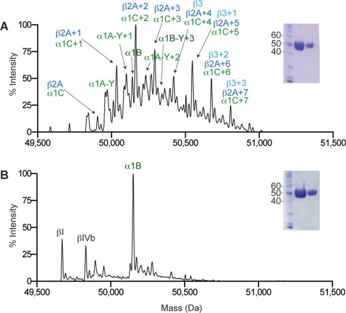
FIGURE 1:
Isoform composition and purity of tubulin isolated from brain tissue and tsA201 cells using the TOG affinity method. (A) Mass spectra and SDSu2013polyacrylamide gel (inset) of tubulin isolated from mo...
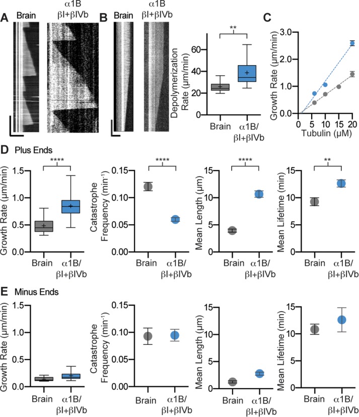
FIGURE 2:
Dynamics of brain and u03b11B/u03b2I+u03b2IVb microtubules. (A) Kymographs showing typical microtubule growth for brain and u03b11B/u03b2I+u03b2IVb tubulin at 6 u00b5M. Horizontal and vertical scale b...
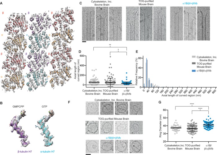
FIGURE 3:
Cryoelectron microscopy of u03b11B/u03b2I+u03b2IVb microtubules. (A) Cross-section of the cryo-EM map (gray density) and model of GMPCPP human u03b11B/u03b2I+u03b2IVb microtubules (three protofilament...
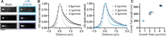
FIGURE 4:
EB1-GFP comet analysis on brain and u03b11B/u03b2I+u03b2IVb microtubules. (A) TIRF microscopy images of EB1-GFP comets at the ends of growing brain microtubules (left) and u03b11B/u03b2I+u03b2IVb (rig...
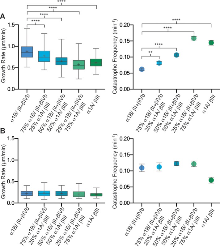
FIGURE 5:
Modulation of u03b11B/u03b2I+u03b2IVb tubulin dynamics by addition of neuronal u03b11A/u03b2III tubulin. (A) Left panel: box-whisker plot (whiskers indicate minimum and maximum) showing plus-end growt...
Figure images are served from the NIH/NLM PubMed Central Open Access Subset or Europe PMC; copyright remains with the publishers and authors.
💬 Discussion
0 commentsNo comments yet. Be the first to start a discussion!
Leave a Comment