Abstract
Drosophila melanogaster is a model organism rich in genetic tools to manipulate and identify neural circuits involved in specific behaviors. Here we present a technique for two-photon calcium imaging in the central brain of head-fixed Drosophila walking on an air-supported ball. The ball's motion is tracked at high resolution and can be treated as a proxy for the fly's own movements. We used the genetically encoded calcium sensor, GCaMP3.0, to record from important elements of the motion-processing pathway, the horizontal-system lobula plate tangential cells (LPTCs) in the fly optic lobe. We presented motion stimuli to the tethered fly and found that calcium transients in horizontal-system neurons correlated with robust optomotor behavior during walking. Our technique allows both behavior and physiology in identified neurons to be monitored in a genetic model organism with an extensive repertoire of walking behaviors.
🔬 Techniques
🧬 Organisms
💻 Software
✨ Fluorophores
🧪 Sample Preparation
🏭 Microscope Brands
🧪 Reagent Suppliers
🔴 Lasers
📷 Detectors
🎨 Filters
💻 Software Details
💾 Data Repositories
🏛️ Research Organizations (ROR)
Affiliated research institutions:
📋 Methods
Fly stocks
Flies were reared on standard cornmeal agar under a 12-hr light/12-hr dark cycle at 25° C. All experiments were performed on adult female flies, 2–4 days post-eclosion. Stocks were generously provided as follows: R27B03-Gal4 (Gerry Rubin, Aljoscha Nern), UAS-GCaMP3.0 (Loren Looger, Julie Simpson). Line R27B03 was constructed by the methods described in Pfeiffer et al. 2008 45 and identified as driving expression in the HS-neurons by A. Nern (unpublished). Fly holder The details of the holder geometry are shown in Supplementary Figs. 1 and 2a . The lower side of the fly holder is painted black using a metal staining opaque paint (Dykem opaque staining, ITW Dymon, KS) to avoid reflections of the visual stimulus on the shim surface that could affect the fly’s behavioral responses. This holder is robust and reusable. Fly preparation and positioning on the ball A female fly was anesthetized on ice and transferred onto a cold plate. We fixed the extended proboscis of the fly with a wax mixture (1:1 molten bee wax and colophony, Sigma Aldrich 60895) to minimize motion of the brain. Under a dissection microscope we glued a pin to the anterior third of the fly’s thorax at a 45–60° angle, and inserted the pin into a mount attached to a three-axis micromanipulator to position the fly’s head and thorax in the holder. This was done above a cold stage to minimize fly movement. The head of the fly was bent forward by about 70–80° to give access to its posterior surface, and glued to the holder with UV-activated glue (Fotoplast Gel, Dreve, part number 44691). The glue was spread along the head using a pulled glass capillary with a small glass ball of about 40 μm diameter at its end. The glue was cured after each step using UV light (LED-100 UV portable, Electro-lite Corp) for about 20 s. After gluing the head, the fly was lowered slightly using the micromanipulator and moved backwards to relax neck tension and give good optical access to the dorsal part of the head and the LPTCs ( Supplementary Fig. 2b ). Any uncured glue at the surface was removed using a paper tissue and extensive rinsing with saline. Under saline solution 46 with 2mM Ca 2+ , we used sharpened #5 forceps to carefully remove the cuticle and some of the fat tissue preventing optical access to the LPTCs (see Supplementary Fig. 2b ). Calcium signals can easily be lost if the neural processes are damaged during the dissection. We also removed the muscle, M16 10 , to prevent brain motion. The procedure lasted about 40 minutes. Most flies that were fixed in the holder did not immediately show walking behavior after positioning on the ball. Consistent walking behavior (e.g., as shown in Supplementary Movie 1 ) developed soon after the fly adapted to the ball. The adaptation is mostly due to the positioning of the fly in the holder. If flies are adapted to the ball they quickly begin walking behavior after the dissection and can maintain it for up to 4 hours afterwards (e.g., see Supplementary Fig. 7 ). Treadmill ball Previous Drosophila walking experiments on an air-supported ball have used a Styrofoam ball with a diameter of 7–9 mm and a weight of 10 mg 47 , 30 . When testing a Styrofoam ball with these specifications we noticed that flies easily lifted the ball. We used a ball of 40 mg (6 mm diameter) manufactured out of polyurethane foam (Last-A-Foam, FR7120, General Plastics Manufacturing Company) using a bowl shaped file with an inner diameter of 6 mm ( Supplementary Fig. 8a ). The edge of the file is sharp and the radial surface is textured using electrical discharge machining (EDM). This results in a surface texture similar to a nail file. With the ball file inserted into a hand-held drill, a piece of polyurethane foam was slowly rotated against the ball file until it became a sphere with a diameter of 6 mm. The ball can be coated with polyurethane spray paint to prevent small dust particles from coming off the ball. Ball holder, flow meter The ball floats on a stream of air 30 . The ball holder has a hemispherical bowl for the ball, shown schematically in Supplementary Fig. 8b . The bowl is lightly smoothed using a glass bead abrasion machine. The airflow was adjusted using a flowmeter (correlated flowmeter, max. flow rate: 825 mL/min, Cole-Parmer, EW-3227-16). High-resolution ball tracker To track the movement of the air-supported ball, we developed a custom high-speed “optical flow camera” based on a commercially available motion sensing chip (Avago Technologies ADNS-6090). The ADNS-6090 measures optical flow based on sequential correlations of 30×30 pixel images, with a maximum frame rate of 7.2 kHz. The ADNS-6090 can acquire snapshot video frames of its visual field and stream the pixel data at video rates (20 Hz). Our camera system consists of three discrete units: Two cubical camera enclosures with c-mount lens threads, and a single MCU base unit to which the cameras are connected via 10 wire ribbon cables ( Supplementary Fig. 9 ). Tracker: Microcontroller core, signal conditioning, signal I/O, and power The interface between the ADNS-6090 and the PC was mediated by a deterministic microcontroller with a 20 MHz quartz oscillator. The controller responds to commands from the PC user, acquires data at a fixed sample rate, and conditions data for return to the PC or to the real-time interface. The Atmel ATMega644p is at the core of our system. Firmware was developed for the Atmel microcontroller in the CodeVisionAVR C development environment and programmed to the device via a USB in-system programmer (Atmel AVR ISP mkII). The MCU was driven at 5 V, provided by the USB data cable, for TTL logic level compatibility through the real-time interface. Conversion to 3.3 V logic for communication with the ADNS sensor chip was accomplished with non-inverting precision Schmitt-triggers. The MCU communicates with the ADNS-6090 via a 6-line serial interface. This interface operates at 3.3 V, and is clocked in a custom serial “bit-banging” fashion in order to send identical data to both chips while reading responses from the cameras on separate parallel lines. The bit stream can be paused and continued during operation. Serial port communication with a PC is accomplished via a UART to USB converter (FTDI FT232BL). In our implementation, the serial interface operates with a data rate of 1Mbit/sec. An analog representation of the motion signals (accumulated over a user-selectable fixed time interval) was generated on 4 external lines for each of the four principal axis velocities during operation. Four channels of analog output are provided by a 12-bit parallel 4-channel digital to analog converter. This parallel addressed device allows for simultaneous latching of output values to prevent sample phase lag across output channels. Tracker: Firmware state machine and data packet format The majority of the firmware code for the MCU consists of a user interface state machine that responds to multiple byte commands from the PC user. Fixed byte commands control the state of the system in either “Idle,” “Video Streaming,” or ”Motion Data Streaming” modes. Other commands allow for a communications bridge between the PC user and the internal configuration and status registers of the ADNS-6090. Data streaming to a PC is timed by a dedicated interrupt service routine driven by the system quartz oscillator signal. During the data read from the cameras, the MCU services UART transmit interrupts so as to deliver data to the PC user while concurrently acquiring new data from the ADNS-6090 chips in an interleaved fashion. The serial data stream consists of packets containing a header byte, a counter byte that loops over the 0–255 range, and a programmable number of bytes including X/Y velocity values from each camera or combined pitch/roll/yaw/blank values (4 bytes), camera surface quality values (2 bytes), and 16-bit shutter speed values (4 bytes). The overall system sample rate is primarily limited by the time to read values from the ADNS camera chips and may be increased by reducing the data packet size. Tracker: Camera housing, mounting frame, lenses, & illumination The ADNS sensor is delivered with a bushing that is designed to direct light onto the chip from an integrated illumination source at a prescribed angle to the package in typical optical mouse applications. The bushing may be removed by releasing a set of plastic tabs at either end of the long axis of the package. The plastic frame of the chip is soldered in place so as to be flush against the back surface of a circuit board ( Supplementary Fig. 10a ) mounted inside a custom anodized aluminum frame ( Supplementary Fig. 10b ). We visualized the moving surface through a 25 mm CCTV lens, a 2x lens extender, and a 1 inch extension tube. Tracker: Calibration and optical alignment of the tracking system To align the tracking cameras we used a cubical target that fits into the air support stand. We calibrated the tracking system and tested the linearity of the motion measurement by directly controlling the rotational velocity of the ball. The ball was attached to a servo motor (Compumotor SM161AE-NGSN, controlled by a Gemini GV Servo Drive, Parker Motion Control Systems, Rohnert Park, CA), which rotated at constant velocities for different durations. We derived a velocity calibration factor by comparing the velocities measured with the tracking system to known (command) ball velocities ( Supplementary Fig. 11a ). The calibration was well fit by a linear regression, with a coefficient of regression of 0.99 (clockwise rotations, n = 10; counterclockwise rotations, n=10). Moreover, the calibration factor was constant across all tested velocities. We examined the precision of the system by testing its performance during movement onsets and stops. The tracker responded reliably across all velocities tested with a tick for every 80 μms at the magnification used ( Supplementary Fig. 11b ). Further, simultaneous movement tracking with two cameras gave identical results in all trials (median difference across different displacements = 0, range form −1 to 1 arbitrary units, n = 40, Supplementary Fig. 11c ). Tracking performance depends on shutter speed and surface quality, which in turn depend on illumination conditions. We used 850-nm collimated IR LEDs with flexible arms (SLFA-850-12-2-SA-110, Illumination Control, Inc.) illuminating the ball from a distance of 1–2 cm roughly parallel to the optical axis of the tracking cameras without obstructing the field of view to achieve the highest surface quality and shutter speeds (see Supplementary Fig. 12 ). We ensured the consistency of tracking conditions by recording the ball’s movement at a frame rate of 480 Hz at the beginning of each experiment using a third camera (camera 3 in Fig. 1b ). This camera was placed directly behind the fly and had a similar field of view as the tracking cameras, with a resolution set to 100×100 pixels. We compared the ball’s trajectory as determined by the tracking system to that obtained by the extra camera using offline MATLAB image processing code based on subimage cross-correlations. We found a linear relationship between calibration factors computed from ball tracker output and camera-measured translation (R 2 = 0.99 ± 0.004, see Supplementary Fig. 11d ). Given the close agreement between X and Y calibration factors (6.6 ± 0.6 and 6.1 ± 0.6 respectively), we used the average of the two for the rotational calibration factor. Tracker: Reconstruction of the fly’s walking trajectories We used two tracking cameras (Camera 1 and Camera 2 in Fig. 2a ) to acquire the ball’s three rotational degrees of freedom, roll, pitch, and yaw. The cameras were positioned at the equator of the ball at a distance of 8 to 10 cm, and at 135° and −135° in the azimuth, with 0° degrees corresponding to the fly’s body axis (in the ideal alignment condition, brown arrow in Fig. 2a, b ). Both cameras tracked motion of the ball using their local view, measuring movement in the x (X 1 and X 2 ) and y (Y 1 and Y 2 ,) directions. We then extracted yaw (pure rotation of the fly, referred to as rotational velocity or velocity_rotation), pitch (velocity_forward) and roll (velocity_side) velocities as follows: velocity _ forward ball = ( Y 1 + Y 2 ) ∗ cos ( γ ) , with γ = 45 ° , and velocity _ side ball = ( Y 1 − Y 2 ) ∗ sin ( γ ) , velocity _ rotation ball = ( X 1 + X 2 ) / 2. Ball movement compensates for the fly’s walking motion, and ball velocities therefore translate directly to virtual velocities of the fly. Thus: velocity _ forward fly = − velocity _ forward ball velocity _ side fly = − velocity _ side ball velocity _ rotation fly = − velocity _ rotation ball . We defined translational velocities as the square root of the sum of the squares of forward and side velocities. To reconstruct the fly’s virtual 2-dimensional trajectory we used both position and gaze. Briefly, for a coordinate system centered on the fly with a y-axis along the fly’s body axis at its first position (0,0,0), if the fly’s current coordinates on a virtual flat plane are (fly x , fly y , θ), its new position is: θ new = θ + velocity _ rotation fly × Δ t fly xnew = fly x + velocity _ side fly ∗ cos ( θ new ) − velocity _ forward fly ∗ sin ( θ new ) fly ynew = fly y + velocity _ side fly ∗ sin ( θ new ) + velocity _ forward fly ∗ cos ( θ new ) . Tracker: MATLAB software user interface The MATLAB-based interface software provides two functions: control/calibration, and data streaming/logging. One component is a visualization tool that streams the visual fields of the cameras (2×30×30 = 1800 pixels) at a 20 Hz frame rate. The tracker data are either displayed in a 2D field as independent points or applied as rotational transformations to a 3D ball. The data path to and from the PC is mediated either via a virtual serial COM port or direct access to the FTDI D2xx C based driver library. Visual display arena and shielding We used a modular LED arena to present visual stimuli to the fly 32 . The light of the blue LED arena (Bright LED Electronics Corp., emission maximum at 465 nm) had to be filtered to avoid interference with fluorescence detection during two-photon imaging. The arena was covered with four layers of Kodak color filters (Kodak Wratten No 47B). However, filtering was not complete and the remaining fluorescent background due to bleed-through-induced intensity, which peaked at 450 nm (FWHM = 45 nm), was typically 4 ± 2.8% ΔF/F (with respect to baseline fluorescence during arena–off conditions) for a PMT gain of 0.405 V. This offset was ( Supplementary Fig. 3 ) subtracted for each trial (see Data Analysis in Online Methods ). Moreover, in our calcium signal analysis, we defined the baseline during the segment of a stationary (not-moving) pattern (see below). The maximal luminance of the visual arena with the filter was 0.85 cd/m 2 . The semi-cylinder arena was constructed from 14 modular LED panel displays with a resolution of 16×56 pixels, with a height of 70 mm and a diameter of 123 mm. When the fly is positioned at the center, those dimensions span ~157° in azimuth and 45° in elevation with a maximum pixel subtense of 2.8°, all with respect to the fly’s visual field. However, because the fly was on the ball, the subtended angle of elevation was reduced to ~40°. Horizontal moving patterns were generated with vertical bars of constant spatial period (λ = 22.4°) moving at 22.4 °/s so that the temporal frequency (the angular velocity of the pattern divided by the spatial period) was 1Hz. Patterns were generated in which 3 consecutive frames with intermediate intensity levels at the edges of the bars were used to define one pixel displacement. Large-field sine gratings of maximal contrast were presented to the fly in two protocols, which differed only in trial length. The first protocol consisted of a 5-s stationary pattern segment after which the pattern moved in the preferred direction (PD) of the neuron for 10 s. Following PD stimulation, another 5-second stationary pattern segment preceded motion of the pattern in the anti-preferred or null direction (ND) of the neuron for 10 s. The trial ended with 5 s of the stationary pattern. In the second protocol both the stationary and moving segments lasted 15 s. Thus, trials run with Protocol 1 lasted 35 s, whereas trials run with Protocol 2 lasted 75 s.
Show full methods section
Fly stocks
Flies were reared on standard cornmeal agar under a 12-hr light/12-hr dark cycle at 25° C. All experiments were performed on adult female flies, 2–4 days post-eclosion. Stocks were generously provided as follows: R27B03-Gal4 (Gerry Rubin, Aljoscha Nern), UAS-GCaMP3.0 (Loren Looger, Julie Simpson). Line R27B03 was constructed by the methods described in Pfeiffer et al. 2008 45 and identified as driving expression in the HS-neurons by A. Nern (unpublished). Fly holder The details of the holder geometry are shown in Supplementary Figs. 1 and 2a . The lower side of the fly holder is painted black using a metal staining opaque paint (Dykem opaque staining, ITW Dymon, KS) to avoid reflections of the visual stimulus on the shim surface that could affect the fly’s behavioral responses. This holder is robust and reusable. Fly preparation and positioning on the ball A female fly was anesthetized on ice and transferred onto a cold plate. We fixed the extended proboscis of the fly with a wax mixture (1:1 molten bee wax and colophony, Sigma Aldrich 60895) to minimize motion of the brain. Under a dissection microscope we glued a pin to the anterior third of the fly’s thorax at a 45–60° angle, and inserted the pin into a mount attached to a three-axis micromanipulator to position the fly’s head and thorax in the holder. This was done above a cold stage to minimize fly movement. The head of the fly was bent forward by about 70–80° to give access to its posterior surface, and glued to the holder with UV-activated glue (Fotoplast Gel, Dreve, part number 44691). The glue was spread along the head using a pulled glass capillary with a small glass ball of about 40 μm diameter at its end. The glue was cured after each step using UV light (LED-100 UV portable, Electro-lite Corp) for about 20 s. After gluing the head, the fly was lowered slightly using the micromanipulator and moved backwards to relax neck tension and give good optical access to the dorsal part of the head and the LPTCs ( Supplementary Fig. 2b ). Any uncured glue at the surface was removed using a paper tissue and extensive rinsing with saline. Under saline solution 46 with 2mM Ca 2+ , we used sharpened #5 forceps to carefully remove the cuticle and some of the fat tissue preventing optical access to the LPTCs (see Supplementary Fig. 2b ). Calcium signals can easily be lost if the neural processes are damaged during the dissection. We also removed the muscle, M16 10 , to prevent brain motion. The procedure lasted about 40 minutes. Most flies that were fixed in the holder did not immediately show walking behavior after positioning on the ball. Consistent walking behavior (e.g., as shown in Supplementary Movie 1 ) developed soon after the fly adapted to the ball. The adaptation is mostly due to the positioning of the fly in the holder. If flies are adapted to the ball they quickly begin walking behavior after the dissection and can maintain it for up to 4 hours afterwards (e.g., see Supplementary Fig. 7 ). Treadmill ball Previous Drosophila walking experiments on an air-supported ball have used a Styrofoam ball with a diameter of 7–9 mm and a weight of 10 mg 47 , 30 . When testing a Styrofoam ball with these specifications we noticed that flies easily lifted the ball. We used a ball of 40 mg (6 mm diameter) manufactured out of polyurethane foam (Last-A-Foam, FR7120, General Plastics Manufacturing Company) using a bowl shaped file with an inner diameter of 6 mm ( Supplementary Fig. 8a ). The edge of the file is sharp and the radial surface is textured using electrical discharge machining (EDM). This results in a surface texture similar to a nail file. With the ball file inserted into a hand-held drill, a piece of polyurethane foam was slowly rotated against the ball file until it became a sphere with a diameter of 6 mm. The ball can be coated with polyurethane spray paint to prevent small dust particles from coming off the ball. Ball holder, flow meter The ball floats on a stream of air 30 . The ball holder has a hemispherical bowl for the ball, shown schematically in Supplementary Fig. 8b . The bowl is lightly smoothed using a glass bead abrasion machine. The airflow was adjusted using a flowmeter (correlated flowmeter, max. flow rate: 825 mL/min, Cole-Parmer, EW-3227-16). High-resolution ball tracker To track the movement of the air-supported ball, we developed a custom high-speed “optical flow camera” based on a commercially available motion sensing chip (Avago Technologies ADNS-6090). The ADNS-6090 measures optical flow based on sequential correlations of 30×30 pixel images, with a maximum frame rate of 7.2 kHz. The ADNS-6090 can acquire snapshot video frames of its visual field and stream the pixel data at video rates (20 Hz). Our camera system consists of three discrete units: Two cubical camera enclosures with c-mount lens threads, and a single MCU base unit to which the cameras are connected via 10 wire ribbon cables ( Supplementary Fig. 9 ). Tracker: Microcontroller core, signal conditioning, signal I/O, and power The interface between the ADNS-6090 and the PC was mediated by a deterministic microcontroller with a 20 MHz quartz oscillator. The controller responds to commands from the PC user, acquires data at a fixed sample rate, and conditions data for return to the PC or to the real-time interface. The Atmel ATMega644p is at the core of our system. Firmware was developed for the Atmel microcontroller in the CodeVisionAVR C development environment and programmed to the device via a USB in-system programmer (Atmel AVR ISP mkII). The MCU was driven at 5 V, provided by the USB data cable, for TTL logic level compatibility through the real-time interface. Conversion to 3.3 V logic for communication with the ADNS sensor chip was accomplished with non-inverting precision Schmitt-triggers. The MCU communicates with the ADNS-6090 via a 6-line serial interface. This interface operates at 3.3 V, and is clocked in a custom serial “bit-banging” fashion in order to send identical data to both chips while reading responses from the cameras on separate parallel lines. The bit stream can be paused and continued during operation. Serial port communication with a PC is accomplished via a UART to USB converter (FTDI FT232BL). In our implementation, the serial interface operates with a data rate of 1Mbit/sec. An analog representation of the motion signals (accumulated over a user-selectable fixed time interval) was generated on 4 external lines for each of the four principal axis velocities during operation. Four channels of analog output are provided by a 12-bit parallel 4-channel digital to analog converter. This parallel addressed device allows for simultaneous latching of output values to prevent sample phase lag across output channels. Tracker: Firmware state machine and data packet format The majority of the firmware code for the MCU consists of a user interface state machine that responds to multiple byte commands from the PC user. Fixed byte commands control the state of the system in either “Idle,” “Video Streaming,” or ”Motion Data Streaming” modes. Other commands allow for a communications bridge between the PC user and the internal configuration and status registers of the ADNS-6090. Data streaming to a PC is timed by a dedicated interrupt service routine driven by the system quartz oscillator signal. During the data read from the cameras, the MCU services UART transmit interrupts so as to deliver data to the PC user while concurrently acquiring new data from the ADNS-6090 chips in an interleaved fashion. The serial data stream consists of packets containing a header byte, a counter byte that loops over the 0–255 range, and a programmable number of bytes including X/Y velocity values from each camera or combined pitch/roll/yaw/blank values (4 bytes), camera surface quality values (2 bytes), and 16-bit shutter speed values (4 bytes). The overall system sample rate is primarily limited by the time to read values from the ADNS camera chips and may be increased by reducing the data packet size. Tracker: Camera housing, mounting frame, lenses, & illumination The ADNS sensor is delivered with a bushing that is designed to direct light onto the chip from an integrated illumination source at a prescribed angle to the package in typical optical mouse applications. The bushing may be removed by releasing a set of plastic tabs at either end of the long axis of the package. The plastic frame of the chip is soldered in place so as to be flush against the back surface of a circuit board ( Supplementary Fig. 10a ) mounted inside a custom anodized aluminum frame ( Supplementary Fig. 10b ). We visualized the moving surface through a 25 mm CCTV lens, a 2x lens extender, and a 1 inch extension tube. Tracker: Calibration and optical alignment of the tracking system To align the tracking cameras we used a cubical target that fits into the air support stand. We calibrated the tracking system and tested the linearity of the motion measurement by directly controlling the rotational velocity of the ball. The ball was attached to a servo motor (Compumotor SM161AE-NGSN, controlled by a Gemini GV Servo Drive, Parker Motion Control Systems, Rohnert Park, CA), which rotated at constant velocities for different durations. We derived a velocity calibration factor by comparing the velocities measured with the tracking system to known (command) ball velocities ( Supplementary Fig. 11a ). The calibration was well fit by a linear regression, with a coefficient of regression of 0.99 (clockwise rotations, n = 10; counterclockwise rotations, n=10). Moreover, the calibration factor was constant across all tested velocities. We examined the precision of the system by testing its performance during movement onsets and stops. The tracker responded reliably across all velocities tested with a tick for every 80 μms at the magnification used ( Supplementary Fig. 11b ). Further, simultaneous movement tracking with two cameras gave identical results in all trials (median difference across different displacements = 0, range form −1 to 1 arbitrary units, n = 40, Supplementary Fig. 11c ). Tracking performance depends on shutter speed and surface quality, which in turn depend on illumination conditions. We used 850-nm collimated IR LEDs with flexible arms (SLFA-850-12-2-SA-110, Illumination Control, Inc.) illuminating the ball from a distance of 1–2 cm roughly parallel to the optical axis of the tracking cameras without obstructing the field of view to achieve the highest surface quality and shutter speeds (see Supplementary Fig. 12 ). We ensured the consistency of tracking conditions by recording the ball’s movement at a frame rate of 480 Hz at the beginning of each experiment using a third camera (camera 3 in Fig. 1b ). This camera was placed directly behind the fly and had a similar field of view as the tracking cameras, with a resolution set to 100×100 pixels. We compared the ball’s trajectory as determined by the tracking system to that obtained by the extra camera using offline MATLAB image processing code based on subimage cross-correlations. We found a linear relationship between calibration factors computed from ball tracker output and camera-measured translation (R 2 = 0.99 ± 0.004, see Supplementary Fig. 11d ). Given the close agreement between X and Y calibration factors (6.6 ± 0.6 and 6.1 ± 0.6 respectively), we used the average of the two for the rotational calibration factor. Tracker: Reconstruction of the fly’s walking trajectories We used two tracking cameras (Camera 1 and Camera 2 in Fig. 2a ) to acquire the ball’s three rotational degrees of freedom, roll, pitch, and yaw. The cameras were positioned at the equator of the ball at a distance of 8 to 10 cm, and at 135° and −135° in the azimuth, with 0° degrees corresponding to the fly’s body axis (in the ideal alignment condition, brown arrow in Fig. 2a, b ). Both cameras tracked motion of the ball using their local view, measuring movement in the x (X 1 and X 2 ) and y (Y 1 and Y 2 ,) directions. We then extracted yaw (pure rotation of the fly, referred to as rotational velocity or velocity_rotation), pitch (velocity_forward) and roll (velocity_side) velocities as follows: velocity _ forward ball = ( Y 1 + Y 2 ) ∗ cos ( γ ) , with γ = 45 ° , and velocity _ side ball = ( Y 1 − Y 2 ) ∗ sin ( γ ) , velocity _ rotation ball = ( X 1 + X 2 ) / 2. Ball movement compensates for the fly’s walking motion, and ball velocities therefore translate directly to virtual velocities of the fly. Thus: velocity _ forward fly = − velocity _ forward ball velocity _ side fly = − velocity _ side ball velocity _ rotation fly = − velocity _ rotation ball . We defined translational velocities as the square root of the sum of the squares of forward and side velocities. To reconstruct the fly’s virtual 2-dimensional trajectory we used both position and gaze. Briefly, for a coordinate system centered on the fly with a y-axis along the fly’s body axis at its first position (0,0,0), if the fly’s current coordinates on a virtual flat plane are (fly x , fly y , θ), its new position is: θ new = θ + velocity _ rotation fly × Δ t fly xnew = fly x + velocity _ side fly ∗ cos ( θ new ) − velocity _ forward fly ∗ sin ( θ new ) fly ynew = fly y + velocity _ side fly ∗ sin ( θ new ) + velocity _ forward fly ∗ cos ( θ new ) . Tracker: MATLAB software user interface The MATLAB-based interface software provides two functions: control/calibration, and data streaming/logging. One component is a visualization tool that streams the visual fields of the cameras (2×30×30 = 1800 pixels) at a 20 Hz frame rate. The tracker data are either displayed in a 2D field as independent points or applied as rotational transformations to a 3D ball. The data path to and from the PC is mediated either via a virtual serial COM port or direct access to the FTDI D2xx C based driver library. Visual display arena and shielding We used a modular LED arena to present visual stimuli to the fly 32 . The light of the blue LED arena (Bright LED Electronics Corp., emission maximum at 465 nm) had to be filtered to avoid interference with fluorescence detection during two-photon imaging. The arena was covered with four layers of Kodak color filters (Kodak Wratten No 47B). However, filtering was not complete and the remaining fluorescent background due to bleed-through-induced intensity, which peaked at 450 nm (FWHM = 45 nm), was typically 4 ± 2.8% ΔF/F (with respect to baseline fluorescence during arena–off conditions) for a PMT gain of 0.405 V. This offset was ( Supplementary Fig. 3 ) subtracted for each trial (see Data Analysis in Online Methods ). Moreover, in our calcium signal analysis, we defined the baseline during the segment of a stationary (not-moving) pattern (see below). The maximal luminance of the visual arena with the filter was 0.85 cd/m 2 . The semi-cylinder arena was constructed from 14 modular LED panel displays with a resolution of 16×56 pixels, with a height of 70 mm and a diameter of 123 mm. When the fly is positioned at the center, those dimensions span ~157° in azimuth and 45° in elevation with a maximum pixel subtense of 2.8°, all with respect to the fly’s visual field. However, because the fly was on the ball, the subtended angle of elevation was reduced to ~40°. Horizontal moving patterns were generated with vertical bars of constant spatial period (λ = 22.4°) moving at 22.4 °/s so that the temporal frequency (the angular velocity of the pattern divided by the spatial period) was 1Hz. Patterns were generated in which 3 consecutive frames with intermediate intensity levels at the edges of the bars were used to define one pixel displacement. Large-field sine gratings of maximal contrast were presented to the fly in two protocols, which differed only in trial length. The first protocol consisted of a 5-s stationary pattern segment after which the pattern moved in the preferred direction (PD) of the neuron for 10 s. Following PD stimulation, another 5-second stationary pattern segment preceded motion of the pattern in the anti-preferred or null direction (ND) of the neuron for 10 s. The trial ended with 5 s of the stationary pattern. In the second protocol both the stationary and moving segments lasted 15 s. Thus, trials run with Protocol 1 lasted 35 s, whereas trials run with Protocol 2 lasted 75 s.
Free walking behavior
Flies walked on a flat, round platform with a diameter of 95 mm surrounded by a cylindrical arena (360° in azimuth) that was constructed from panels identical to those used for tethered walking. However, the LED light was not filtered, which resulted in a slight green shift of the stimulus light and many times greater stimulus intensity. The walking platform was actively maintained at the same temperature as was used for the tethered experiments (21 °C). The flies were enclosed by a heated metal ring with a height of 3.8 mm that supported a glass plate coated with Sigmacote (Sigma-Aldrich; arena design: T. Ofstad & M. Reiser, unpublished). We placed three 2–4-day old flies at a time on the platform, and presented stationary, clockwise and counterclockwise stimulation with the same pattern used in the tethered walking experiments. Each stimulus condition lasted 15 s and the stimulus sequence was repeated for 20 minutes. We tracked the positions of walking flies at 15 fps with a camera (Basler 602f) from above. We obtained walking trajectories for each fly using Ctrax software 48 , and calculated the translational and rotational velocities based on the distance moved between subsequent frames (75 ms). For averaging, we excluded parts where the fly was stationary (< 1 mm/s translational velocity). Velocities of tethered flies were calculated as the change in position during 75 ms, and were smoothed using Savitzky-Golay filtering with a span of 150 ms.
Two-photon imaging
We imaged on a custom-built two-photon microscope using ScanImage 3.6 software 49 and Olympus water immersion objectives (LUMPlanFl/IR, 60×, N.A. 0.9 and LUMPlanFl/IR, 40x, N.A. 0.8). A mode-locked Ti:Sapphire Chameleon Ultra II laser (Coherent, Santa Clara, CA) tuned to 920–930 nm was used as the excitation source. Fluorescence was collected using photomultiplier tubes (Hamamatsu, Hamamatsu City, Japan) after bandpass filtering using a BG22 emission filter (Chroma Technologies, Brattleboro, VT) and either an HQ615/70–2p filter (Chroma Technologies, Nrattleboro, VT) or FF01-680/SP-25 filter (Semrock). An additional filter was used to minimize bleed through of arena light (FF01-542/50–25, Semrock). Images were acquired in framescan mode (4–16Hz). We noticed that using laser intensity much beyond 20 mW (measured at the back aperture) produced behavioral responses in flies (presumably due to heating 50 ), and subsequently restricted the laser intensity to below 15 mW. We only imaged the left half of the fly brain. Therefore, data presented as HS always refers to the left HS neuron, for which PD corresponds to rotations in the counterclockwise direction. Data analysis: Two-photon imaging Image processing was performed using custom code written and run in MATLAB. To correct motion artifacts during behavior, we implemented image registration of the raw image sequence by translational-compensation-based discrete Fourier analysis (efficient subpixel registration 43 ). In most cases, we needed only minimal motion correction (see Supplementary Fig. 13 ). Regions of interest were selected manually. Peak responses were calculated as the difference between the mean of last second within the PD segment and the mean of the last second within the ND segment. Data analysis: Optomotor behavior We defined an optomotor response index to quantify the optomotor response of the fly as follows: Optomotor Index = ∑ V ccw − ∑ V c w ∑ abs ( V ccw ) + ∑ abs ( V c w ) , with V cw representing rotational velocity signals obtained when the pattern moved clockwise. Similarly V ccw represents rotational velocity signals when the pattern moved counter-clockwise. When the fly “rotates” counterclockwise (i.e., when the ball rotates clockwise), the animal’s rotational velocity signals are positive. Conversely, when the fly “rotates” clockwise (i.e. the ball rotates counterclockwise), the rotational velocity signals are negative. The index ranges from 1 (pure optomotor response) to −1 (pure counter-optomotor response). Data analysis: Correlations between neuronal and behavioral responses After selecting trials in which flies showed positive O.I., cross-correlations were computed between behavioral responses (rotations) and fluorescence transients during PD stimulation. If zero-lag correlations were found to be negative, as was only rarely the case, we show cross-covariance minima in Fig. 4g (red trials, numbers of trials in Supplementary Information ). Otherwise, we took the positive peak of cross-covariances. For computing lags, only trials showing positive cross-covariances were used. Lags were computed across trials and flies as the delay between the measured onset of fluorescence response (3 s.d.s greater than baseline) and the onset of behavioral response (angular rotation 3 s.d.s greater than baseline in the direction of motion stimulus). For behavioral responses, we numerically corrected any baseline bias (caused by the fly favoring rotation towards one side over another before a stimulus is presented due to minor imbalances in positioning). We first calculated a bias slope over the entire baseline period across trials, and then used it to compute linear corrections for the entire trace.
Supplementary Material 1 Supplementary Movie M1 Real-time movie shows multiple views of the fly walking in response to visual stimulation. Supplementary Movie M2 Real-time movie shows fly-on-the-ball virtual 2D trajectory during 2-photon imaging trial in response to counterclockwise (blue) and then clockwise (red) global horizontal motion of vertical stripes (1 Hz spatial frequency). The frame rate is chosen to show fly’s movements in real time. Frame size in X: 30 mm; Y: 45 mm. Supplementary Movie M3 Real-time movie shows a second example of fly-on-the-ball virtual 2D trajectory during 2-photon imaging trial in response to counterclockwise (blue) and then clockwise (red) global horizontal motion of vertical stripes (1 Hz spatial frequency). The frame rate is chosen to show fly’s movements in real time. Frame size in X: 35 mm; Y: 40 mm. Supplementary Movie M4 Real-time movie shows (clockwise from top-left): GCaMP signal from R27B03-Gal4 HS-neuron soma (shown in false color, linear intensity scale, window size: X = 62 μm, Y = 67 μm); visual pattern presented to the fly (motion is first in the null direction for the HS-neuron, and then in the preferred direction); view of fly walking on ball from camera 3 (behind fly); traces of change in %ΔF/F (in green) and accumulated rotation (in black) as the motion stimuli are presented. Two-photon images are unfiltered (aside from xvid compression applied to entire movie) and not motion-corrected. Supplementary Movie M5 Real-time movie shows (clockwise from top-left): GCaMP signal from R27B03-Gal4 HS-neuron dendrites (false color, linear intensity scale, window size: 43 μm); visual pattern presented to the fly (motion is first in the null direction for the HS-neuron, then in the preferred direction and this protocol is repeated); view of fly walking on ball from camera 3 (behind fly); traces of change in %ΔF/F (in green) and accumulated rotation (in black) as the motion stimuli are presented. Two-photon images are unfiltered (aside from xvid compression of the movie) and not motion- corrected.
📊 Figures
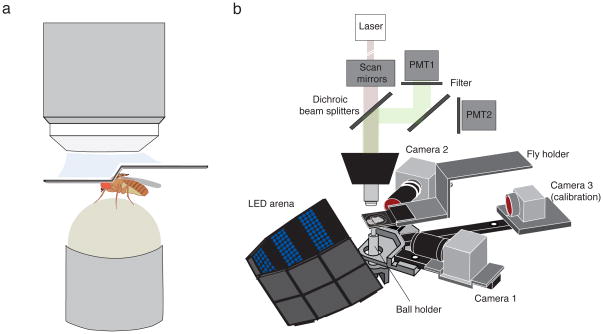
Figure 1
Setup for two-photon imaging from the brain of head-fixed flies walking on a ball
( a ) Fly holder for tethered walking fly recording separates exposed brain from intact legs and eyes allowing visual stimulation and walking on the ball. ( b ) Schematic showing arrangement of holder...
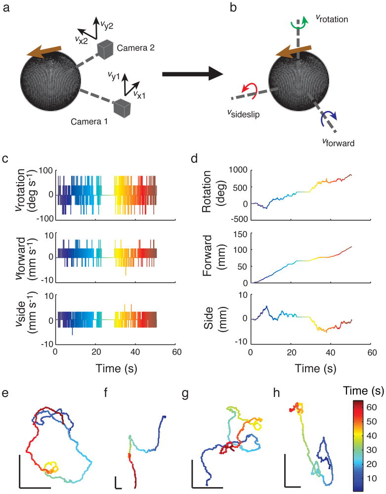
Figure 2
High-precision ball tracking system allows online measurement of flyu2019s virtual trajectory
( a ) Both cameras capture X and Y velocity in their respective fields of view. Together, they provide 4 kHz tracking of the ballu2019s rotation about all three axes. The brown arrow shows the flyu201...
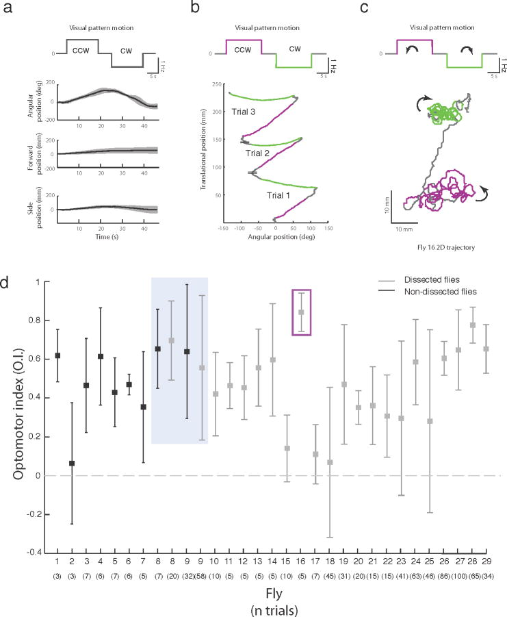
Figure 3
Optomotor behavior in tethered flies
( a ) Rotational and translational velocity of one fly in response to clockwise (CCW) and counterclockwise (CW) motion stimuli. The flyu2019s rotational velocity, plotted as mean u00b1 s.d., n = 5 tri...
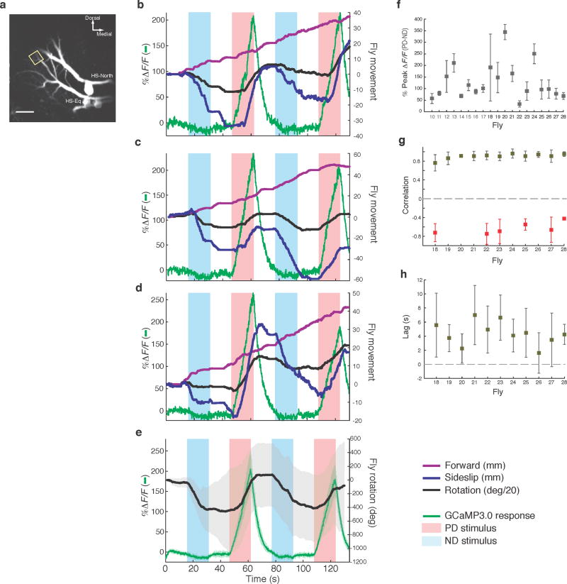
Figure 4
Optical imaging of dendrites of a motion-sensitive neuron during tethered walking
( a ) Typical Z-projected image of HS-neurons expressing GCaMP3.0 ( R27B03-Gal4 ). Only HS-North and HS-Equatorial are clearly visible. The rectangle outlines a typical distal dendritic region of inte...
Figure images are served from the NIH/NLM PubMed Central Open Access Subset or Europe PMC; copyright remains with the publishers and authors.
💬 Discussion
0 commentsNo comments yet. Be the first to start a discussion!
Leave a Comment