Abstract
We introduce field synthesis, a theorem and method that can be used to synthesize any scanned or dithered light sheet, including those used in lattice light-sheet microscopy (LLSM), from an incoherent superposition of one-dimensional intensity distributions. Compared to LLSM, this user-friendly and modular approach offers a simplified optical design, higher light throughput and simultaneous multicolor illumination. Further, field synthesis achieves lower rates of photobleaching than light sheets generated by lateral beam scanning.
🔬 Techniques
✨ Fluorophores
🧪 Sample Preparation
🔬 Cell Lines
🏭 Microscope Brands
🔴 Lasers
📷 Detectors
🔎 Objectives
🎨 Filters
💻 Software Details
💻 Code & Software
💾 Data Repositories
🏛️ Research Organizations (ROR)
Affiliated research institutions:
📋 Methods
Microscope Setup
The basic units to generate lattice and field synthesis light-sheets are shown in Figure S1 and our microscope setup is illustrated in Figure S11 . A 488 (Sapphire 488–300 LP, Coherent) and a 561 nm (OBIS 561–150LS, Coherent) are combined with a dichroic mirror (LM01–503-25, Semrock), and focused through a 50-micron spatial filter (P25H, ThorLabs) with a 50 mm focal length achromatic lens (AC254–050-A, Thorlabs). Thereafter, flip mirror 1 is used to select either the LLSM or Field Synthesis optical paths, and the beam is recollimated with a 75 (AC254–075-A, Thorlabs) or 400 (AC508–400-A, Thorlabs) mm focal length achromatic lens, respectively. Further, the optical system is operated in a fluorescence (e.g., with orthogonal detection, Figure S11A ) or transmission (e.g., with diascopic detection, Figure S11B ) mode, to image fluorescent specimens and investigate light-sheet properties, respectively. The LLSM path is a simplified version of the original set-up. 1 The collimated and expanded beam is further magnified and shaped to a line beam by a pair of achromatic cylindrical lenses (68–160, Edmund optics and ACY254–200-A, Thorlabs). The line beam uniformly illuminates a region on the spatial light modulator (SLM, SXGA-3DM, Forth Dimension Displays) where the lattice pattern is displayed. A polarized beamsplitter (10FC16PB.3, Newport) and a half-wave plate (AHWP10M-600, Thorlabs) are placed in front of the SLM, and together with the SLM form the pattern generator. 5 , 20 The lasers were assembled in a way that the polarization states fit the pattern generator. The diffraction light from the SLM is focused by an achromatic lens (AC508–400-A, Thorlabs) on a custom-designed mask (mask 1, Photo Sciences, Inc.). The mask has various annuli to block unwanted diffraction orders (mainly the 0 th order but also higher orders). Different sizes of the annuli correspond to different outer and inner NAs on the back focal plane of the illumination objective lens. After passing through the mask, the desired diffraction orders are de-magnified through two achromatic lenses (AC254–150-A, AC254–100-A, Thorlabs) and fit into the size of a galvanometer (Galvo mirror, 6215H, Cambridge Technology). A folding mirror, an achromatic lens (AC-254–100-A, Thorlabs), the flip mirror 2 and a tube lens (ITL-200, Thorlabs) then direct the light to the illumination objective lens (40X, NA0.8, 3.5mm WD, CFI Apo 40XW NIR, Nikon) to form a light-sheet in sample space. All distances between a pair of lenses equal to the summation of their focal lengths so any pair of lenses forms a 4f arrangement. Thus, The SLM is conjugated to the focal plane of the illumination objective lens. The mask is at the Fourier plane of the SLM and is conjugated to the back focal plane of the objective lens. As the galvanometer is conjugated to the mask and the back focal plane of the objective lens, it scans the light-sheet laterally (y) on the focal plane of the detection objective, i.e. enables rapid lateral scanning of a Gaussian or Bessel light-sheet and the dithered mode of the lattice light-sheet. Figure S7 shows typical lattice interference patterns that we could obtain with our setup. The Field synthesis path consists of an iris (IDA20, Thorlabs), an achromatic cylindrical lens (ACY254–050-A, Thorlabs), an achromatic lens (AC254–075-A, Thorlabs), another custom-designed mask (mask 2), and a tube lens (ITL-200, Thorlabs). An alternative beam expander design to illuminate efficiently smaller field of views is discussed in Supplementary Note 4 and Figure S12 . A galvanometer (Galvo mirror, 6215H, Cambridge Technology) and a folding mirror are placed in between the achromatic cylindrical lens and the achromatic lens. The Galvo mirror is conjugated to the sample plane, which is a similar configuration as used in mSPIM. 21 This path shares the same final tube lens and illumination objective lens with the lattice LSFM path. All distances between a pair of lenses equal to the summation of their focal lengths so any pair of lenses forms a 4f arrangement. The galvanometer in the Field Synthesis path is conjugated to the focal plane of the illumination objective lens. The mask is conjugated to the back focal plane of the objective lens, which is conjugated to the same plane as the mask in the Lattice LSFM path. Since the magnification between the mask and the back focal plane of the objective lens is different in the Field Synthesis LSFM path and the Lattice LSFM path, the sizes of the annuli on mask 2 are designed to match the outer and inner NAs resulted from the annuli on mask 1, as shown in Supplementary Table 2 . The detection path is orthogonal to the illumination path as in a conventional LSFM set-up and it consists of an detection objective lens (40X, NA0.8, 3.5mm WD, CFI Apo 40XW NIR, Nikon), a tube lens (ITL-200, Thorlabs), a dichroic mirror (Di03-R561-t3–25×36, Semrock) that separates the green and the red fluorescence, and two identical sCMOS cameras (Orca Flash4.0 v2, Hamamatsu). A red fluorescence emission filter (FF01–593/LP-25, Semrock) and a green fluorescence emission filter (ET525/50m, Chroma) is placed in front of camera 1 and camera 2, respectively. A piezo stage (P621.1CD, Physik Instrumente) is used to move the sample diagonally to the detection axis in the fluorescence mode ( Figure S11A ) or move the detection objective lens in the transmission mode ( Figure S11B ). In the transmission mode ( Figure S11B ), the detection objective lens is placed along the propagation of the light-sheet and an achromatic lens (AC508–400-A, Thorlabs) is used as the tube lens. An ND filter (ND40A, Thorlabs) is placed in front of the sCMOS camera (Orca Flash4.0 v2, Hamamatsu) to reduce the intensity of the straight light from the lasers. The combination of the 400mm tube lens and the 40x objective lens offers a final magnification of 80x, which results in one pixel on the camera corresponds to 81.25 nm and that can present the light-sheet with a reasonable contrast and resolution. By stepping the detection objective lens with the piezo stage through the illumination lattice, we investigate and measure the 3D light-sheet properties. The pattern on the back focal plane of the excitation objective lens can be observed by Camera 4 (DCC1545M, Thorlabs) with an ND filter (ND10A or ND20A, Thorlabs) in the front when flipped mirror 3 is used. Two achromatic lenses (AC254–100-A and AC254–050-A, Thorlabs) are used to image the back focal plane of the objective lens, which is conjugated to the plane of the masks, on the camera. By observing the pattern on this plane allows us to verify the final outer and inner NAs from both masks and adjust the scan range of the galvo in Field Synthesis.
Show full methods section
Microscope Setup
The basic units to generate lattice and field synthesis light-sheets are shown in Figure S1 and our microscope setup is illustrated in Figure S11 . A 488 (Sapphire 488–300 LP, Coherent) and a 561 nm (OBIS 561–150LS, Coherent) are combined with a dichroic mirror (LM01–503-25, Semrock), and focused through a 50-micron spatial filter (P25H, ThorLabs) with a 50 mm focal length achromatic lens (AC254–050-A, Thorlabs). Thereafter, flip mirror 1 is used to select either the LLSM or Field Synthesis optical paths, and the beam is recollimated with a 75 (AC254–075-A, Thorlabs) or 400 (AC508–400-A, Thorlabs) mm focal length achromatic lens, respectively. Further, the optical system is operated in a fluorescence (e.g., with orthogonal detection, Figure S11A ) or transmission (e.g., with diascopic detection, Figure S11B ) mode, to image fluorescent specimens and investigate light-sheet properties, respectively. The LLSM path is a simplified version of the original set-up. 1 The collimated and expanded beam is further magnified and shaped to a line beam by a pair of achromatic cylindrical lenses (68–160, Edmund optics and ACY254–200-A, Thorlabs). The line beam uniformly illuminates a region on the spatial light modulator (SLM, SXGA-3DM, Forth Dimension Displays) where the lattice pattern is displayed. A polarized beamsplitter (10FC16PB.3, Newport) and a half-wave plate (AHWP10M-600, Thorlabs) are placed in front of the SLM, and together with the SLM form the pattern generator. 5 , 20 The lasers were assembled in a way that the polarization states fit the pattern generator. The diffraction light from the SLM is focused by an achromatic lens (AC508–400-A, Thorlabs) on a custom-designed mask (mask 1, Photo Sciences, Inc.). The mask has various annuli to block unwanted diffraction orders (mainly the 0 th order but also higher orders). Different sizes of the annuli correspond to different outer and inner NAs on the back focal plane of the illumination objective lens. After passing through the mask, the desired diffraction orders are de-magnified through two achromatic lenses (AC254–150-A, AC254–100-A, Thorlabs) and fit into the size of a galvanometer (Galvo mirror, 6215H, Cambridge Technology). A folding mirror, an achromatic lens (AC-254–100-A, Thorlabs), the flip mirror 2 and a tube lens (ITL-200, Thorlabs) then direct the light to the illumination objective lens (40X, NA0.8, 3.5mm WD, CFI Apo 40XW NIR, Nikon) to form a light-sheet in sample space. All distances between a pair of lenses equal to the summation of their focal lengths so any pair of lenses forms a 4f arrangement. Thus, The SLM is conjugated to the focal plane of the illumination objective lens. The mask is at the Fourier plane of the SLM and is conjugated to the back focal plane of the objective lens. As the galvanometer is conjugated to the mask and the back focal plane of the objective lens, it scans the light-sheet laterally (y) on the focal plane of the detection objective, i.e. enables rapid lateral scanning of a Gaussian or Bessel light-sheet and the dithered mode of the lattice light-sheet. Figure S7 shows typical lattice interference patterns that we could obtain with our setup. The Field synthesis path consists of an iris (IDA20, Thorlabs), an achromatic cylindrical lens (ACY254–050-A, Thorlabs), an achromatic lens (AC254–075-A, Thorlabs), another custom-designed mask (mask 2), and a tube lens (ITL-200, Thorlabs). An alternative beam expander design to illuminate efficiently smaller field of views is discussed in Supplementary Note 4 and Figure S12 . A galvanometer (Galvo mirror, 6215H, Cambridge Technology) and a folding mirror are placed in between the achromatic cylindrical lens and the achromatic lens. The Galvo mirror is conjugated to the sample plane, which is a similar configuration as used in mSPIM. 21 This path shares the same final tube lens and illumination objective lens with the lattice LSFM path. All distances between a pair of lenses equal to the summation of their focal lengths so any pair of lenses forms a 4f arrangement. The galvanometer in the Field Synthesis path is conjugated to the focal plane of the illumination objective lens. The mask is conjugated to the back focal plane of the objective lens, which is conjugated to the same plane as the mask in the Lattice LSFM path. Since the magnification between the mask and the back focal plane of the objective lens is different in the Field Synthesis LSFM path and the Lattice LSFM path, the sizes of the annuli on mask 2 are designed to match the outer and inner NAs resulted from the annuli on mask 1, as shown in Supplementary Table 2 . The detection path is orthogonal to the illumination path as in a conventional LSFM set-up and it consists of an detection objective lens (40X, NA0.8, 3.5mm WD, CFI Apo 40XW NIR, Nikon), a tube lens (ITL-200, Thorlabs), a dichroic mirror (Di03-R561-t3–25×36, Semrock) that separates the green and the red fluorescence, and two identical sCMOS cameras (Orca Flash4.0 v2, Hamamatsu). A red fluorescence emission filter (FF01–593/LP-25, Semrock) and a green fluorescence emission filter (ET525/50m, Chroma) is placed in front of camera 1 and camera 2, respectively. A piezo stage (P621.1CD, Physik Instrumente) is used to move the sample diagonally to the detection axis in the fluorescence mode ( Figure S11A ) or move the detection objective lens in the transmission mode ( Figure S11B ). In the transmission mode ( Figure S11B ), the detection objective lens is placed along the propagation of the light-sheet and an achromatic lens (AC508–400-A, Thorlabs) is used as the tube lens. An ND filter (ND40A, Thorlabs) is placed in front of the sCMOS camera (Orca Flash4.0 v2, Hamamatsu) to reduce the intensity of the straight light from the lasers. The combination of the 400mm tube lens and the 40x objective lens offers a final magnification of 80x, which results in one pixel on the camera corresponds to 81.25 nm and that can present the light-sheet with a reasonable contrast and resolution. By stepping the detection objective lens with the piezo stage through the illumination lattice, we investigate and measure the 3D light-sheet properties. The pattern on the back focal plane of the excitation objective lens can be observed by Camera 4 (DCC1545M, Thorlabs) with an ND filter (ND10A or ND20A, Thorlabs) in the front when flipped mirror 3 is used. Two achromatic lenses (AC254–100-A and AC254–050-A, Thorlabs) are used to image the back focal plane of the objective lens, which is conjugated to the plane of the masks, on the camera. By observing the pattern on this plane allows us to verify the final outer and inner NAs from both masks and adjust the scan range of the galvo in Field Synthesis.
Microscope control and image acquisition
The data acquisition computer was equipped with an Intel Xeon E5–2687W v3 processor operating at 3.1GHz with 10 cores and 20 threads, 128GB of 2133MHz DDR4 RAM, and an integrated Intel AHCI chipset controlling 4× 512GB SSDs in a RAID0 configuration. All software was developed using a 64-bit version of LabView 2016 equipped with the LabView Run-Time Engine, Vision Development Module, Vision Run-Time Module and all appropriate device drivers, including NI-RIO Drivers (National Instruments). Software communicated with the camera (Flash 4.0, Hamamatsu) via the DCAM-API for the Active Silicon Firebird frame-grabber and delivered a series of deterministic TTL triggers with a field programmable gate array (PCIe 7852R, National Instruments). These triggers included analog outputs for control of mirror galvanometers, piezoelectric actuators, laser modulation and blanking, camera fire and external trigger, and triggering of the ferroelectric spatial light modulator. A timing diagram for the galvanometric beams scanning in Field Synthesis illustrated in Figure S13 . All images were saved in the OME-TIFF format. 22 Some of the core functions and routines in the microscope control software are licensed under a material transfer agreement from Howard Hughes Medical Institute, Janelia Farm Research Campus. The control software code for Field Synthesis can be requested from the corresponding authors and will be distributed in accordance with this material transfer agreement.
Data Analysis
Image analysis was performed with Fiji 3 and MATLAB (Mathworks). To evaluate the rate of photobleaching for 100 nm fluorescent microspheres, the average intensity of 11 similarly bright beads were measured through time by recording their peak intensity at every timepoint. To this end, a MATLAB script was written that detected the peak intensity of all beads in the dataset and a subset was manually selected that yielded the same average initial intensity for both imaging modalities. The same script was used to initially calibrate the power levels that yielded similar fluorescent counts when the same sample region was imaged with either Bessel beam or Field Synthesis light-sheets. Both the bead imaging as well as the EB3 imaging in the U2OS cells was conducted with such calibrated power levels.
Deconvolution and data post processing
The point spread function (PSF) used for deconvolution of the lattice light-sheet (conventional and Field Synthesis) data was synthesized by using the PSF Generator plugin in ImageJ. 23 , 24 The Born and Wolf 3D optical model is used to generating the PSF.
Illumination and detection
PSFs are synthesized in 3D with the practical experimental parameters (i.e. the refractive index, the wavelength, the NA, and the voxel size). The final light-sheet PSF is the product of the illumination and detection PSFs. Since our sample is placed diagonally to the illumination and detection and we scan the sample to acquire the images (sample-scan acquisition), the light-sheet PSF is sheared oppositely referring to the direction of the sample scan. 3D-deconvolution was performed with 10 iterations of the Richardson-Lucy algorithm as implemented in MATLAB. The deconvolved data was sheared at an angle of 45 degrees using an affine transform and bleach corrected with Fiji using the histogram matching method. For microtubule +TIP data, experimental point-spread functions were obtained by imaging isolated 100 nm nanospheres with both the conventional Bessel and Field Synthesis modes of microscope operation. We chose experimental PSFs here as the Bessel beam light-sheet has a more complex structure and hence could not be approximated with the numerical PSF Generator. These data were deconvolved, the Z-axis bicubically interpolated so that the voxel dimensions were isotropic (162.5 nm) and sheared at an angle of 45 degrees using an affine transform. The EB3 data was not bleach corrected.
Biological Sample Preparation
Both metastatic melanoma (MV3, a kind gift from Dr. Peter Friedl, MD Anderson Cancer Center) and osteosarcoma (U2OS, a kind gift from Dr. Dick McIntosh, University of Colorado Boulder) cell lines were cultured in DMEM supplemented with 10% fetal bovine serum and penicillin/streptomycin and maintained at 37 degrees Celsius with 5% CO 2 atmosphere. MV3 cells were lentivirally transduced using the pLVX-IRES-PURO and pLVX-IRES-NEO expression systems. The GFP-AktPH probe contains GFP fused to the PH domain of Akt and the td-Tomato membrane marker contains td-Tomato fused to the first 60 base pairs of neuromodulin. U2OS cells were lentivirally transduced with a modified pLVX-shRNA2 vector with a truncated CMV promoter to reduce ectopic expression, as previously described. 5 SK-Mel2 cells (a kind gift from Dr. David Drubin, University of California Berkeley) stably expressing CLC-RFP from their native loci were engineered using Zinc-Fingers and TALENS, cultured in DMEM/F12 supplemented with 10% fetal calf serum at 37 degrees Celsius with 5% CO 2 atmosphere. All cells were plated on 5 mm coverslips and mounted in a custom sample holder for imaging. 6 Quantification of Beam Geometry For direct measurements of the light-sheet intensity distribution, the excitation light was imaged in transmission with a 40x water-dipping objective, which was scanned in the Y-direction (e.g., along the optical axis) with a 100-micron piezo actuator. Using a 400 mm tube lens ( Figure S11B ), the effective pixel size of the imaged beam was 81.25 nm. Beam analysis software, written in MATLAB, identified the laser focus in Y, the size of the beam waist in Z and the beam propagation length in Y. Since Bessel and lattice light-sheets are propagation invariant (i.e. they maintain their beam profile over extended propagation distances), we did not apply the Rayleigh length criterion to characterize the light-sheets. Instead, we use the full width half maximum in the propagation direction.
Sequential Lattice data
We developed a simple experiment, which can be reproduced by anyone who has access to a lattice light-sheet microscope, to test the Field synthesis theorem. We termed the procedure sequential lattice: Here, we used the lattice light-sheet illumination path in the square lattice mode and manually positioned a mask to only transmit isolated diffraction orders along the kz direction (see also Figure S2 ). This was repeated for three mask positions and the corresponding datasets were added numerically. As the summing of the intensity is incoherent, at no point a 2D lattice pattern emerges, but only one-dimensional intensity patterns are created. Compared to the dithered square lattice, the sequential lattice approach produces the same light-sheets (see Figure S2 ). In particular, some sidelobe structures are more closely reproduced than in Figure 1D and E . We believe that these small differences arise from slightly different intensity distributions in the pupil plane. Overall, this further confirms that a dithered lattice light-sheet can be synthesized by purely one-dimensional functions, as predicted by the Field Synthesis theorem.
Fluorescent measurement of light-sheet properties
We have characterized the light-sheets using transmission measurements ( Figures 1 and S11B ), which provided images of the light-sheets in sample plane. Due to the involved imaging operation, blurring of the observed light-sheet can be expected, but we argue that this effect will equally affect the conventional and Field Synthesis light-sheets. Nevertheless, we also conducted a direct measurement of the light-sheet in sample space. To this end, we mechanically scanned a 50nm fluorescent bead in 0.2micron steps in the Z-direction and in one-micron steps in the Y-direction through a light-sheet. At every scan position, a widefield image of the fluorescent emission from the bead was taken and the signal on the camera was summed up on a local window surrounding the bead. The window size was chosen such that it contained all diffraction rings of the bead at the largest defocus it was undergoing during the scan. The obtained intensity distributions of a square lattice and a Field Synthesis square lattice light-sheet are shown in Figure S4 . The width of the light sheet at its waist was 0.85 microns for the square lattice and 0.91 microns for the Field synthesis light-sheet. In the propagation direction, the Full width half maximum for the square lattice light-sheet was 16.7 microns and 17.2 microns for the Field Synthesis light-sheet, respectively. These values are in close agreement with the transmission measurements shown in Supplementary Table 3 and the blurring in the transmission measurement appears to be small.
Statistics and Reproducibility
For statistical analysis, we report the mean, standard deviation, and number of observations. To characterize the Bessel, Lattice, and Field Synthesis light-sheets, each light-sheet was spatially averaged across six different regions for multiple repetitions of the imaging experiment (n=2–4, see Table S3 ). In the main and Supplementary Figures, only the averaged light-sheet (the mean) is shown, whereas in Supplementary Table 3 , the mean and standard deviation of the light-sheet parameters are provided. To further test reproducibility, each Lattice and Field Synthesis light-sheet was imaged eight times in transmission and was automatically processed with a Matlab script. We found similar parameters for beam waist and length to the reported values in this manuscript. The fluorescence-based measurement of the lattice and field synthesis light-sheets was also repeated eight times for each mode. We inspected the data visually and measured beam waist and length and found that the results were similar. To compare the photobleaching of a digitally scanned Bessel beam and Field Synthesis, the peak intensity of 11 individual beads was evaluated. In Figure 2C , the mean and 95 th confidence interval for each time point is shown. Likewise, to compare photobleaching of a Lattice Light-Sheet Microscope and Field Synthesis, the peak intensity of 11 isolated beads was evaluated, and the mean and 95 th confidence interval for each time point is shown in Supplementary Figure 9 . To compare the effect of photo-bleaching on EB3, four cells were imaged for each illumination mode. EB3 comets were automatically detected and their average intensity through time measured. Both numerically as visually, the photobleaching was found to be similar to the results shown in Figure 2A & B . For the MV3 cells, at least seven cells were imaged in each mode and similar bleb and filopodia dynamics were observed. On the particular MV3 cells that is shown in Figure 2 , three filopodia blurring events were observed in the sequential lattice mode and none in the simultaneous field synthesis mode. For the resolution measurements on the clathrin-coated pits, we imaged five different cells for lattice and field synthesis. On the two cells we selected for visualization, we measured 10 well isolated pits for each imaging mode and computed the mean and the standard deviation of the full width half maximum in the axial direction. On the other cells, we manually measured axial profiles with ImageJ and found similar values as reported in supplementary figure S10 .
Data Availability
The datasets acquired for this study are available from the corresponding author upon request. Code Availability The Matlab code is available under https://github.com/AdvancedImagingUTSW/FieldSynthesis The instrument control software can be requested for academic use from the corresponding authors and will be delivered under material transfer agreements with HHMI and UT Southwestern Medical Center.
Supplementary Material 1 video 5 video 6 2 3 4 Supplementary Software video 1 video 2 video 3 video 4
📊 Figures
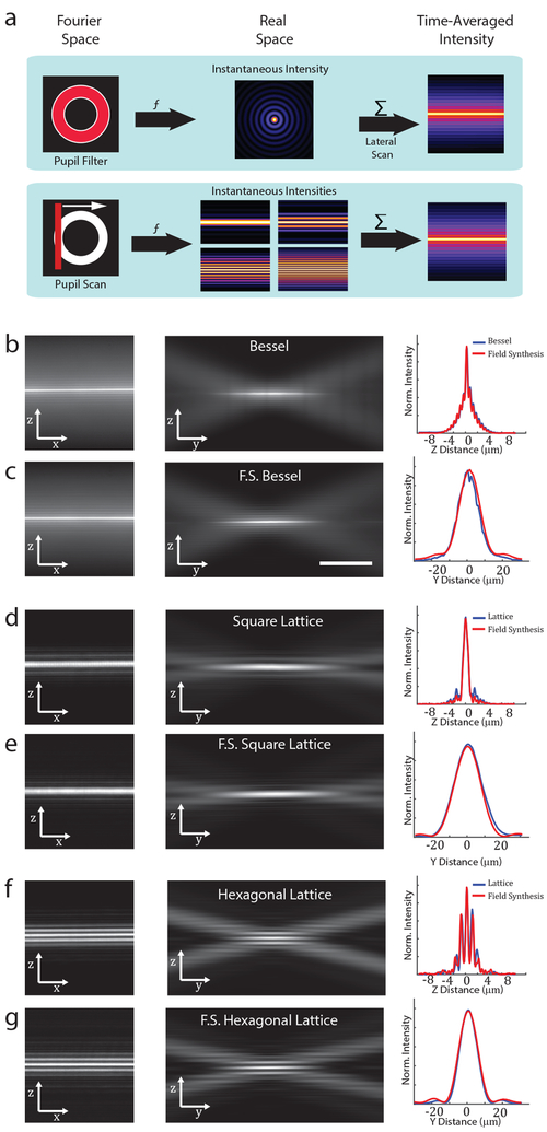
Figure 1
Light-sheet generation by field synthesis. A, Top. In light-sheet microscopy, a pupil filter conjugate to the back-pupil plane of the illumination objective is used to shape the instantaneous laser fo...
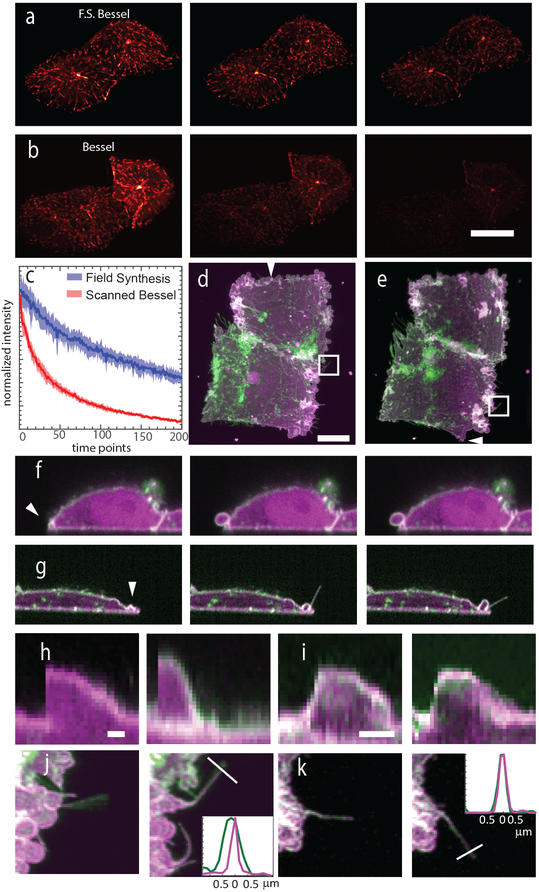
Figure 2
Field Synthesis reduces photobleaching and enables simultaneous multicolor imaging. A. Three timepoints (first, fifteenth, and thirtieth) of a movie of EB3 in an U2OS cell as imaged with Field Synthes...
Figure images are served from the NIH/NLM PubMed Central Open Access Subset or Europe PMC; copyright remains with the publishers and authors.
💬 Discussion
0 commentsNo comments yet. Be the first to start a discussion!
Leave a Comment