Abstract
A long-standing goal of neuroscience has been to understand how computations are implemented across large-scale brain networks. By correlating spontaneous activity during "resting states" [1], studies of intrinsic brain networks in humans have demonstrated a correspondence with task-related activation patterns [2], relationships to behavior [3], and alterations in processes such as aging [4] and brain disorders [5], highlighting the importance of resting-state measurements for understanding brain function. Here, we develop methods to measure intrinsic functional connectivity in Drosophila, a powerful model for the study of neural computation. Recent studies using calcium imaging have measured neural activity at high spatial and temporal resolution in zebrafish, Drosophila larvae, and worms [6-10]. For example, calcium imaging in the zebrafish brain recently revealed correlations between the midbrain and hindbrain, demonstrating the utility of measuring intrinsic functional connections in model organisms [8]. An important component of human connectivity research is the use of brain atlases to compare findings across individuals and studies [11]. An anatomical atlas of the central adult fly brain was recently described [12]; however, combining an atlas with whole-brain calcium imaging has yet to be performed in vivo in adult Drosophila. Here, we measure intrinsic functional connectivity in Drosophila by acquiring calcium signals from the central brain. We develop an alignment procedure to assign functional data to atlas regions and correlate activity between regions to generate brain networks. This work reveals a large-scale architecture for neural communication and provides a framework for using Drosophila to study functional brain networks.
🔬 Techniques
🔭 Microscopes
🧬 Organisms
✨ Fluorophores
🧪 Sample Preparation
🏭 Microscope Brands
🔴 Lasers
📷 Detectors
🎨 Filters
💻 Software Details
📋 Protocols
💻 Code & Software
💾 Data Repositories
🏛️ Research Organizations (ROR)
Affiliated research institutions:
📋 Methods
Overview of data collection and analysis pipeline
To build functional brain networks in Drosophila , we developed a streamlined method of imaging and template registration to reliably extract and compare calcium signals across animals. First, animals that expressed the calcium indicator GCaMP6m[ 13 ] and the red fluorescent protein tdTomato[ 14 ] pan-neuronally were head-fixed, immobilized, and dissected to expose the central brain. Animals were then imaged in the absence of sensory stimuli using a high-speed resonant scanning two-photon system to acquire whole-brain calcium signals (2.6×2.6×7.5μm voxels, 1.91 Hz) and a high-resolution anatomical scan (0.65×0.65×1μm voxels) using the tdTomato signal. We then developed a pipeline to align a standard atlas of annotated brain regions[ 12 ] to each animal’s anatomy using an established template brain[ 15 ]. Finally, after extracting calcium signals from each atlas region, we correlated the time series between each region pair for each fly, providing quantifications of functional connectivity that could be mapped to the current consensus on the position and nomenclature of the fly neuropil.
Analysis of ROI-specific calcium signals
We next correlated the extracted time series between pairs of ROIs ( Figure 2A ). As expected, large calcium excursions that spanned multiple ROIs produced strong correlations ( Figure 2B ). We also observed strong correlations between ROIs that lacked such excursions ( Figure 2C ). Lastly, we observed that some ROIs were not significantly correlated ( Figure 2D ). This demonstrates that correlations between ROIs can arise from multiple features in calcium signals and are selective to particular pairs of ROIs. Examining individual voxel contributions to ROI calcium signals, we found that voxel signals within each ROI were well represented by the average ROI signal and were reasonably homogenous ( Figure 2SA ; Figure S2B ), although future work generating functional connectivity-based atlases could potentially increase signal homogeneity within ROIs.
Show full methods section
Overview of data collection and analysis pipeline
To build functional brain networks in Drosophila , we developed a streamlined method of imaging and template registration to reliably extract and compare calcium signals across animals. First, animals that expressed the calcium indicator GCaMP6m[ 13 ] and the red fluorescent protein tdTomato[ 14 ] pan-neuronally were head-fixed, immobilized, and dissected to expose the central brain. Animals were then imaged in the absence of sensory stimuli using a high-speed resonant scanning two-photon system to acquire whole-brain calcium signals (2.6×2.6×7.5μm voxels, 1.91 Hz) and a high-resolution anatomical scan (0.65×0.65×1μm voxels) using the tdTomato signal. We then developed a pipeline to align a standard atlas of annotated brain regions[ 12 ] to each animal’s anatomy using an established template brain[ 15 ]. Finally, after extracting calcium signals from each atlas region, we correlated the time series between each region pair for each fly, providing quantifications of functional connectivity that could be mapped to the current consensus on the position and nomenclature of the fly neuropil.
Analysis of ROI-specific calcium signals
We next correlated the extracted time series between pairs of ROIs ( Figure 2A ). As expected, large calcium excursions that spanned multiple ROIs produced strong correlations ( Figure 2B ). We also observed strong correlations between ROIs that lacked such excursions ( Figure 2C ). Lastly, we observed that some ROIs were not significantly correlated ( Figure 2D ). This demonstrates that correlations between ROIs can arise from multiple features in calcium signals and are selective to particular pairs of ROIs. Examining individual voxel contributions to ROI calcium signals, we found that voxel signals within each ROI were well represented by the average ROI signal and were reasonably homogenous ( Figure 2SA ; Figure S2B ), although future work generating functional connectivity-based atlases could potentially increase signal homogeneity within ROIs.
Methods for quantifying intrinsic brain network functional connectivity Here, we introduce a pipeline to reliably quantify functional connections between brain regions in Drosophila . Our approach offers three critical advantages. First, it provides a means to align functional data to a common brain template and atlas, allowing datasets to be directly compared. Second, it employs commonly used tools for image registration and analysis that can be widely applied. Third, our analyses demonstrate that intrinsic functional correlations emerge at low frequencies, a phenomenon also observed in fMRI-based connectivity. As a result, it is possible to acquire such functional measurements at high spatial resolution using commercially available laser scanning two-photon microscopes. Our results also suggest that imaging methods with higher spatial resolution may be more useful for this approach than those with greater temporal resolution. Therefore, slower GCaMP variants may be more appropriate for measuring intrinsic connectivity, although this might not be the case for stimulus-dependent connectivity where higher frequency oscillations could dominate. In this case, faster imaging could be combined with a head-fixed setup that allows for freedom of motion to examine how stimuli and behavior alter functional connectivity. Moreover, a finer parcellation of the brain atlas may allow for the identification of functional connections that would otherwise be undetected, such as activity in sub-regions of the ellipsoid body during navigation[ 20 ]. Finally, while our current methodology cannot provide information about the directionality of functional connections, future work using high speed imaging combined with indicators with faster kinetics could allow quantification of directed brain networks.
Applications of functional network analysis in Drosophila While much of our understanding of functional brain networks has come from research in humans, our ability to perform invasive experiments to manipulate networks in humans is limited. We suggest that Drosophila is a powerful model for the study of brain networks. First, individual neurons, clusters of neurons, or whole brain regions can be manipulated, through a combination of genetic and optical methods, on both short and long time scales, allowing us to probe dynamic network changes as individual elements are perturbed. Such experiments could, for example, guide understanding of brain lesions by causally probing the relationship between a lesioned region’s connectivity and changes in network organization[ 28 ]. Second, mutations that affect behavior or model brain disorders in flies could be combined with this approach to use network architecture as a phenotypic readout that extends our mechanistic understanding. In the future, we anticipate that exploring how cellular, genetic, and physiological manipulations alter intrinsic brain network architecture in the fly will make important advances in our understanding of brain organization and behavior.
STAR Methods CONTACT FOR REAGENT AND RESOURCE SHARING
Further information and requests for resources and reagents should be directed to and will be fulfilled by the Lead Contact, Thomas R. Clandinin ( trc@stanford.edu ).
EXPERIMENTAL MODEL AND SUBJECT DETAILS Fly stocks
Strains are provided in the Key Resources Table . All animals used in experiments were females of the genotype w+; UAS-myr::tdTomato/UAS-GCaMP6m; nSyb-Gal4/+ . Flies were raised on molasses medium at 25°C with a 12/12-hour light/dark cycle. Flies were housed in mixed male/female vials and 5-day old females were selected for imaging.
METHOD DETAILS Calcium imaging Preparation
All animals were imaged on the fifth day post-eclosion. Flies were cold-anaesthetized by putting them in an empty vial and chilling them on ice for approximately one minute. Flies were then inserted into a collar that fits around the cervix and provides a separate chamber for the head and the rest of the fly as previously described ( Figure S1N–Q )[ 10 ]. Animals were immobilized using nail polish applied to the back of the head, to the proximal portions of the legs, and to the wings to prevent motion. Nail polish was applied via mouth pipette through a pulled glass capillary, allowing for precise application. Animals were gently dissected in cold fly saline (103 mM NaCl, 3 mM KCl, 5 mM TES, 1 mM NaH2PO4, 4 mM MgCl2, 1.5 mM CaCl2, 10 mM trehalose, 10 mM glucose, 7 mM sucrose, and 26 mM NaHCO3) lacking calcium or sugar. To expose the central brain, the proboscis, antennae, and surrounding cuticle were removed, as were the trachea and fat occluding the brain. The eyes and other cuticle were left intact. Flies were then transferred to a custom mount and perfused with complete saline bubbled with 95% O 2 and 5% CO 2 .
Microscopy
Flies were imaged at room temperature on a Bruker Ultima system with resonant scanning capability, a piezo objective mount, and GaAsP type PMTs using a Leica 20× HCX APO 1.0 NA water immersion objective lens. GCaMP6m signals were excited with a Chameleon Vision II femtosecond laser (Coherent) at 920nm, and collected through a 525/50nm filter. Myr::tdTomato signals were excited at 920nm and collected through a 595/50nm filter. GCaMP6m was selected over other variants as its kinetics best matched our imaging rate. Both channels were collected in resonant scanning mode (8kHz line scan rate, bidirectional scanning). GCaMP6m functional data was volumetrically imaged at a resolution of 128×128 (2.6×2.6μm) with 25 z-sections (7.5μm steps with 2× frame averaging, effective frame rate ~50Hz). For high speed z-sectioning, a piezo mount was used to control the position of objective. Z-stacks were collected unidirectionally. While the entire fly CNS, including the cell body cortex and central neuropils, were imaged in these experiments, only voxels corresponding to the neuropil atlas were used in analyses. Neuropils are highly structured in Drosophila and represent the functional units of the fly CNS. As the central brain of the fly is estimated to have 100,000 neurons that span tens to hundreds of microns in length, with submicron scale processes, each neuron contributed signals to multiple voxels, and each voxel contained the signals from tens of neurons. Each fly was imaged for two 17.4-minute sessions (2000 time points) in the absence of any sensory stimuli. Specifically, the imaging room was temperature controlled (70°F) and flies were imaged in complete darkness. Removal of antennae prevented possible olfactory or auditory inputs. Removal of the proboscis and immobilization of the legs prevented possible gustatory inputs and contact with tastants. Anatomical myr::tdTomato stacks were collected in resonant scanning mode immediately prior to each functional GCaMP6m imaging session. These anatomical scans were collected at a resolution of 512×512 (0.65×0.65μm) with 181 z-sections (1 μm steps with 32× frame averaging).
Data preprocessing Alignment
All alignment was done on the anatomical scan using CMTK, via the munger wrapper with the parameters specified[ 17 ]. Specifically, alignment was performed using the munger parameters (-X 26 –C 8 –G 80 –R 4 –A ‘–accuracy 0.4’ –W ‘–accuracy 0.4’). The atlas was then warped with each specific set of warping parameters using the reformatx command (CMTK) with the –nn (nearest neighbor) flag to prevent errors in the edge assignment of the atlas. Both the template and the atlas used can be downloaded from the virtual fly brain project website ( www.virtualflybrain.org ). For the generation of the mean brain, eight myr::tdTomato anatomical scans (collected as stated above), not included in our experimental dataset, were aligned to each other (seven brains to one seed brain) using the same CMTK parameters. The seed brain was determined by selecting the best aligned single anatomical scan from multiple flies and was collected with a voxel resolution of 0.62×0.62×0.6 μm. The process of averaging brains aligned to the seed brain to generate the mean brain produced better alignment to the template than the seed brain alone (data not shown). An average of each voxel was taken by loading these as a 4D hyper-stack in ImageJ and taking the mean value across the eight brains.
Motion correction
Functional data was motion corrected using the 3dvolreg command in AFNI[ 29 ]. First, a mean functional dataset for each fly was created by averaging the first 100 volumes, using AFNI’s 3dTstat command. To perform motion correction, each functional volume was then aligned to the mean functional using 3dvolreg. Each dataset was inspected visually for quality of motion correction and confirmation that the motion-corrected functional data was aligned to the live structural data. Data exclusion Data was excluded from both imaging runs (i.e., data not included in analyses presented here, N = 6) or one imaging run (N = 8) prior to calculation of correlation matrices for several reasons. These included data that could not be adequately aligned to the template brain, functional data that drifted beyond our initial imaging bounds in any dimension during the imaging session, excessive motion in functional data, and animals in which the esophagus or other structure occluded any part of the brain. Additionally, fourteen atlas ROIs were not included in our functional connectivity analyses because we either did not image them in total (i.e., optic lobe ROIs, medulla, lobula, lobula plate, and accessory medulla) or the erosion process eliminated them from any single fly in our dataset, usually a result of their small size (i.e., bulb, cantle, left inferior posterior slope, left gall).
Functional connectivity and network analyses
ROI erosion ROIs were eroded by one voxel (using the 3dmask_tool command in AFNI) after resampling them to functional resolution (using the 3dresample command in AFNI) to prevent incorrect assignment of edge voxels to ROIs. Erosion by one voxel was chosen to approximate our alignment error ( Figure 1 ) and was limited by the fact that further erosion eliminated many ROIs.
Quantification of functional connectivity
Using the 3dmaskave command in AFNI, we then extracted calcium imaging signals from all voxels in an ROI and then averaged the time series across these voxels to produce a single time series for each ROI in each fly. We next computed correlations of the time series between each ROI pair using Pearson’s correlations and applying a Fisher z-transform to generate 61 × 61 correlation matrices for each fly that represent functional connectivity between ROIs. ROI homogeneity was calculated with two methods. First, for each ROI and fly, we calculated the Pearson’s correlation between the time series of each voxel in that ROI and the average time series of that ROI (‘Voxel-Mean’; Figure S2A ). Second, for each ROI and fly, we calculated the Pearson’s correlations between each voxel pair in that ROI (‘Voxel-Voxel’; Figure S2B ). For each method, we then Fisher z-transformed the resulting correlation values and averaged across the voxels within each ROI to provide a summary statistic for each ROI and fly. One ROI in one fly was excluded from further analysis because it contained only one voxel. Reliability of correlation matrices between and within flies was examined by quantifying the correlation of functional connectivity values across datasets. First, to examine reliability between animals, correlations of functional connectivity values were computed between all possible pairs of flies (N = 18 flies, N = 153 inter-animal correlations) and were averaged over all pairs. Second, to examine reliability within flies, we collected two imaging runs (N = 2000 timepoints each) on a subset of flies (N = 10). Correlations of functional connectivity values were computed between the two imaging runs for each fly and then averaged. Examination of intrinsic network properties We next examined various properties of functional connectivity to characterize large-scale intrinsic network organization in the fly brain. First, to examine the significance of individual functional connections across all animals, we conducted one-sample t-tests against a comparison value of zero on the Fisher-transformed correlation values for each connection pair across flies, to identify functional connections with significant positive or negative correlation values. We used stringent significance threshold of α = 0.001, Bonferroni-corrected for all functional connection pairs (N = 1830 possible connections for 61 brain regions; p < 5.46e–7). Second, we examined how functional connectivity strength differs depending on the hemispheric-location of functional connections. For each fly, we quantified right and left intra-hemispheric functional connectivity by averaging correlation values (i.e., Fisher z-transformed values) within all right (N = 28 ROIs) and left-hemisphere (N = 26 ROIs) regions, respectively. We quantified inter-hemispheric functional connectivity by averaging correlation values between all right- and left-hemisphere region pairs. We quantified homologous pair functional connectivity by averaging correlation values between the same brain regions in the opposite hemispheres (N = 26 ROI pairs). We quantified midline functional connectivity by averaging correlation values between midline regions (N = 7 ROIs) and all other brain regions. To examine whether functional connectivity strength differed across these five categories, we conducted a repeated-measures ANOVA with a within-subjects factor of lateralization category. Post-hoc comparisons between category pairs were conducted with paired-samples t-tests. Third, we examined regional differences in the number of functional connections between midline and lateral regions (e.g., number of significant functional connections passing a corrected p < 0.001). For each of the seven midline regions, we calculated the number of its functional connections to lateral (non-midline) regions. To examine whether these 71 functional connections were uniformly distributed across the seven midline regions, we conducted a chi-squared test on the number of lateral functional connections for each midline region.
Generation of simulated data and spectral analyses
To confirm that the observed significant functional connections were not spuriously caused by our imaging methods or sampling rate, we generated simulated time series based on properties of our real data from N = 18 flies. Specifically, for each fly, we generated ROI-specific time series of random data with the same mean and standard deviation as the real ROI time series. To simulate data with similar temporal properties as our calcium imaging signal, we convolved these simulated time series with the kinetic profile of GCaMP6m[ 13 ] ( Figure S3B ) using a sum of exponentials: f ( x ) = e - 0.696 x - e - 4.5 x In particular, the initial random data were scaled such that the simulated data had the same mean and standard deviation as the real ROI time series after convolution. We repeated this procedure 1000 times for each fly, thus generating a dataset of 18000 simulated time series for each ROI. For each simulated dataset, we computed the Pearson’s correlations between each ROI pair and applied a Fisher z-transform. Using an identical significance threshold as the real data, we then quantified the number of significant functional connections in each simulated dataset. To examine the spectral properties of our data in relationship to our imaging methods, we applied a series of temporal filters (fifth-order Butterworth) spanning 0.1–0.9 Hz in 0.1 Hz steps to the ROI time series for each fly. After computing correlations between each ROI pair and applying a Fisher z-transform, we quantified the average functional connectivity across all ROI pairs. We then compared the average functional connectivity value for each filter to that from the unfiltered data ( Figure S3D ). We also computed the coherence, the spectral analog of cross-correlation, between each ROI pair for each fly ( Figure S3E ).
QUANTIFICATION AND STATISTICAL ANALYSIS
Quantification of ROI Homogeneity
Significance of ROI homogeneity was tested with one-sample t-tests of the average Fisher-transformed correlation values against a comparison value of 0 for N = 18 files. As this analysis was exploratory in nature, we report significant ROI functional connectivity that passes a p < 8.20e-4 threshold (α = 0.05, Bonferroni-corrected for 61 ROIs tested). Results are presented in Figures 2A and 2B and include mean ± SEM across flies.
Identification of functional connections
Significance of individual functional connection pairs was tested with one-sample t-tests of the Fisher-transformed correlation values against a comparison value of 0 for N = 18 flies. We report significant functional connections that pass a p < 5.46e-7 threshold (α = 0.001, Bonferroni corrected for 1830 comparisons for all possible ROI pairs). Results are presented in Figure 3A and include mean Fisher-transformed correlation values across flies. A similar approach was taken to identifying significant functional connections during data simulations. Example simulated data are presented in Figures S3A and S3C and include ROI time series and mean Fisher-transformed correlation values across flies, respectively. Significance of ROI functional connectivity (i.e., average functional connectivity of each ROI to the remaining 60 ROIs) was tested with one-sample t-tests of the average Fisher-transformer correlation values against a comparison value of 0 for N = 18 files. We report significant ROI functional connectivity that passes a p < 1.64e-5 threshold (α = 0.001, Bonferroni-corrected for 61 ROIs tested). Results are presented in Figure 3B and include mean ± SEM across flies. Relationship between ROI size and connectivity Correlations between ROI size and connectivity were calculated with Pearson’s correlations between the number of voxels in each ROI (averaged over flies) and (1) ROI functional connectivity (i.e., functional connectivity of each ROI to the remaining 60 ROIs, averaged over flies) and (2) the number of significant functional connections of each ROI. Results are presented in the Results section. Examination of connectivity lateralization Differences in functional connectivity depending on hemispheric location were tested with a repeated-measures ANOVA with a within-subjects factor of connectivity type (intra-hemispheric left, intra-hemispheric right, inter-hemispheric, homologous pairs, midline) for N = 18 flies. Post-hoc comparisons were conducted with paired-samples t-tests. Results are presented in Figure 4B and include mean ± SEM across flies (left) and individual flies (right). The ANOVA was performed in Prism. Differences in the distribution of significant midline functional connections were conducted with a chi-squared test of the number of functional connections (N = 71) across the seven midline regions. All statistical tests were two-tailed. Significant midline connections are presented in Figure 4C .
DATA AND SOFTWARE AVAILABILITY
Data illustrating the alignment pipeline as well as sample functional imaging data and atlas ROIs can be found on Mendeley Data ( http://dx.doi.org/10.17632/8b6nw2xxhn.1 ). Code using Python, AFNI[ 29 ], and FSL[ 30 ] to process functional data and generate ROI time series can be found at: https://github.com/cgallen/MannGallen_2017_CurrentBiology .
EXPERIMENTAL MODEL AND SUBJECT DETAILS Fly stocks
Strains are provided in the Key Resources Table . All animals used in experiments were females of the genotype w+; UAS-myr::tdTomato/UAS-GCaMP6m; nSyb-Gal4/+ . Flies were raised on molasses medium at 25°C with a 12/12-hour light/dark cycle. Flies were housed in mixed male/female vials and 5-day old females were selected for imaging.
METHOD DETAILS Calcium imaging Preparation
All animals were imaged on the fifth day post-eclosion. Flies were cold-anaesthetized by putting them in an empty vial and chilling them on ice for approximately one minute. Flies were then inserted into a collar that fits around the cervix and provides a separate chamber for the head and the rest of the fly as previously described ( Figure S1N–Q )[ 10 ]. Animals were immobilized using nail polish applied to the back of the head, to the proximal portions of the legs, and to the wings to prevent motion. Nail polish was applied via mouth pipette through a pulled glass capillary, allowing for precise application. Animals were gently dissected in cold fly saline (103 mM NaCl, 3 mM KCl, 5 mM TES, 1 mM NaH2PO4, 4 mM MgCl2, 1.5 mM CaCl2, 10 mM trehalose, 10 mM glucose, 7 mM sucrose, and 26 mM NaHCO3) lacking calcium or sugar. To expose the central brain, the proboscis, antennae, and surrounding cuticle were removed, as were the trachea and fat occluding the brain. The eyes and other cuticle were left intact. Flies were then transferred to a custom mount and perfused with complete saline bubbled with 95% O 2 and 5% CO 2 .
Microscopy
Flies were imaged at room temperature on a Bruker Ultima system with resonant scanning capability, a piezo objective mount, and GaAsP type PMTs using a Leica 20× HCX APO 1.0 NA water immersion objective lens. GCaMP6m signals were excited with a Chameleon Vision II femtosecond laser (Coherent) at 920nm, and collected through a 525/50nm filter. Myr::tdTomato signals were excited at 920nm and collected through a 595/50nm filter. GCaMP6m was selected over other variants as its kinetics best matched our imaging rate. Both channels were collected in resonant scanning mode (8kHz line scan rate, bidirectional scanning). GCaMP6m functional data was volumetrically imaged at a resolution of 128×128 (2.6×2.6μm) with 25 z-sections (7.5μm steps with 2× frame averaging, effective frame rate ~50Hz). For high speed z-sectioning, a piezo mount was used to control the position of objective. Z-stacks were collected unidirectionally. While the entire fly CNS, including the cell body cortex and central neuropils, were imaged in these experiments, only voxels corresponding to the neuropil atlas were used in analyses. Neuropils are highly structured in Drosophila and represent the functional units of the fly CNS. As the central brain of the fly is estimated to have 100,000 neurons that span tens to hundreds of microns in length, with submicron scale processes, each neuron contributed signals to multiple voxels, and each voxel contained the signals from tens of neurons. Each fly was imaged for two 17.4-minute sessions (2000 time points) in the absence of any sensory stimuli. Specifically, the imaging room was temperature controlled (70°F) and flies were imaged in complete darkness. Removal of antennae prevented possible olfactory or auditory inputs. Removal of the proboscis and immobilization of the legs prevented possible gustatory inputs and contact with tastants. Anatomical myr::tdTomato stacks were collected in resonant scanning mode immediately prior to each functional GCaMP6m imaging session. These anatomical scans were collected at a resolution of 512×512 (0.65×0.65μm) with 181 z-sections (1 μm steps with 32× frame averaging).
Data preprocessing Alignment
All alignment was done on the anatomical scan using CMTK, via the munger wrapper with the parameters specified[ 17 ]. Specifically, alignment was performed using the munger parameters (-X 26 –C 8 –G 80 –R 4 –A ‘–accuracy 0.4’ –W ‘–accuracy 0.4’). The atlas was then warped with each specific set of warping parameters using the reformatx command (CMTK) with the –nn (nearest neighbor) flag to prevent errors in the edge assignment of the atlas. Both the template and the atlas used can be downloaded from the virtual fly brain project website ( www.virtualflybrain.org ). For the generation of the mean brain, eight myr::tdTomato anatomical scans (collected as stated above), not included in our experimental dataset, were aligned to each other (seven brains to one seed brain) using the same CMTK parameters. The seed brain was determined by selecting the best aligned single anatomical scan from multiple flies and was collected with a voxel resolution of 0.62×0.62×0.6 μm. The process of averaging brains aligned to the seed brain to generate the mean brain produced better alignment to the template than the seed brain alone (data not shown). An average of each voxel was taken by loading these as a 4D hyper-stack in ImageJ and taking the mean value across the eight brains.
Motion correction
Functional data was motion corrected using the 3dvolreg command in AFNI[ 29 ]. First, a mean functional dataset for each fly was created by averaging the first 100 volumes, using AFNI’s 3dTstat command. To perform motion correction, each functional volume was then aligned to the mean functional using 3dvolreg. Each dataset was inspected visually for quality of motion correction and confirmation that the motion-corrected functional data was aligned to the live structural data. Data exclusion Data was excluded from both imaging runs (i.e., data not included in analyses presented here, N = 6) or one imaging run (N = 8) prior to calculation of correlation matrices for several reasons. These included data that could not be adequately aligned to the template brain, functional data that drifted beyond our initial imaging bounds in any dimension during the imaging session, excessive motion in functional data, and animals in which the esophagus or other structure occluded any part of the brain. Additionally, fourteen atlas ROIs were not included in our functional connectivity analyses because we either did not image them in total (i.e., optic lobe ROIs, medulla, lobula, lobula plate, and accessory medulla) or the erosion process eliminated them from any single fly in our dataset, usually a result of their small size (i.e., bulb, cantle, left inferior posterior slope, left gall).
Functional connectivity and network analyses
ROI erosion ROIs were eroded by one voxel (using the 3dmask_tool command in AFNI) after resampling them to functional resolution (using the 3dresample command in AFNI) to prevent incorrect assignment of edge voxels to ROIs. Erosion by one voxel was chosen to approximate our alignment error ( Figure 1 ) and was limited by the fact that further erosion eliminated many ROIs.
Quantification of functional connectivity
Using the 3dmaskave command in AFNI, we then extracted calcium imaging signals from all voxels in an ROI and then averaged the time series across these voxels to produce a single time series for each ROI in each fly. We next computed correlations of the time series between each ROI pair using Pearson’s correlations and applying a Fisher z-transform to generate 61 × 61 correlation matrices for each fly that represent functional connectivity between ROIs. ROI homogeneity was calculated with two methods. First, for each ROI and fly, we calculated the Pearson’s correlation between the time series of each voxel in that ROI and the average time series of that ROI (‘Voxel-Mean’; Figure S2A ). Second, for each ROI and fly, we calculated the Pearson’s correlations between each voxel pair in that ROI (‘Voxel-Voxel’; Figure S2B ). For each method, we then Fisher z-transformed the resulting correlation values and averaged across the voxels within each ROI to provide a summary statistic for each ROI and fly. One ROI in one fly was excluded from further analysis because it contained only one voxel. Reliability of correlation matrices between and within flies was examined by quantifying the correlation of functional connectivity values across datasets. First, to examine reliability between animals, correlations of functional connectivity values were computed between all possible pairs of flies (N = 18 flies, N = 153 inter-animal correlations) and were averaged over all pairs. Second, to examine reliability within flies, we collected two imaging runs (N = 2000 timepoints each) on a subset of flies (N = 10). Correlations of functional connectivity values were computed between the two imaging runs for each fly and then averaged. Examination of intrinsic network properties We next examined various properties of functional connectivity to characterize large-scale intrinsic network organization in the fly brain. First, to examine the significance of individual functional connections across all animals, we conducted one-sample t-tests against a comparison value of zero on the Fisher-transformed correlation values for each connection pair across flies, to identify functional connections with significant positive or negative correlation values. We used stringent significance threshold of α = 0.001, Bonferroni-corrected for all functional connection pairs (N = 1830 possible connections for 61 brain regions; p < 5.46e–7). Second, we examined how functional connectivity strength differs depending on the hemispheric-location of functional connections. For each fly, we quantified right and left intra-hemispheric functional connectivity by averaging correlation values (i.e., Fisher z-transformed values) within all right (N = 28 ROIs) and left-hemisphere (N = 26 ROIs) regions, respectively. We quantified inter-hemispheric functional connectivity by averaging correlation values between all right- and left-hemisphere region pairs. We quantified homologous pair functional connectivity by averaging correlation values between the same brain regions in the opposite hemispheres (N = 26 ROI pairs). We quantified midline functional connectivity by averaging correlation values between midline regions (N = 7 ROIs) and all other brain regions. To examine whether functional connectivity strength differed across these five categories, we conducted a repeated-measures ANOVA with a within-subjects factor of lateralization category. Post-hoc comparisons between category pairs were conducted with paired-samples t-tests. Third, we examined regional differences in the number of functional connections between midline and lateral regions (e.g., number of significant functional connections passing a corrected p < 0.001). For each of the seven midline regions, we calculated the number of its functional connections to lateral (non-midline) regions. To examine whether these 71 functional connections were uniformly distributed across the seven midline regions, we conducted a chi-squared test on the number of lateral functional connections for each midline region.
Generation of simulated data and spectral analyses
To confirm that the observed significant functional connections were not spuriously caused by our imaging methods or sampling rate, we generated simulated time series based on properties of our real data from N = 18 flies. Specifically, for each fly, we generated ROI-specific time series of random data with the same mean and standard deviation as the real ROI time series. To simulate data with similar temporal properties as our calcium imaging signal, we convolved these simulated time series with the kinetic profile of GCaMP6m[ 13 ] ( Figure S3B ) using a sum of exponentials: f ( x ) = e - 0.696 x - e - 4.5 x In particular, the initial random data were scaled such that the simulated data had the same mean and standard deviation as the real ROI time series after convolution. We repeated this procedure 1000 times for each fly, thus generating a dataset of 18000 simulated time series for each ROI. For each simulated dataset, we computed the Pearson’s correlations between each ROI pair and applied a Fisher z-transform. Using an identical significance threshold as the real data, we then quantified the number of significant functional connections in each simulated dataset. To examine the spectral properties of our data in relationship to our imaging methods, we applied a series of temporal filters (fifth-order Butterworth) spanning 0.1–0.9 Hz in 0.1 Hz steps to the ROI time series for each fly. After computing correlations between each ROI pair and applying a Fisher z-transform, we quantified the average functional connectivity across all ROI pairs. We then compared the average functional connectivity value for each filter to that from the unfiltered data ( Figure S3D ). We also computed the coherence, the spectral analog of cross-correlation, between each ROI pair for each fly ( Figure S3E ).
Supplementary Material 1 2 Table S1. Atlas region names, abbreviations, and groupings. Related to Figure 3 Table of atlas regions. Left, regions sorted according to their atlas index. Right, regions sorted alphabetically by name.
📊 Figures
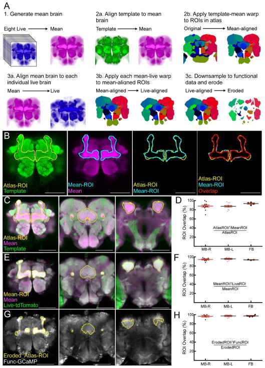
Figure 1
Alignment of brain atlas to functional brain data
(A) Schematic of three-step brain alignment. (1) Eight anatomical scans of a myr:tdTomato channel from live animals were aligned to each other and averaged to generate the u201cmeanu201d brain. (2a) T...
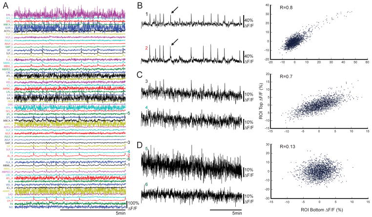
Figure 2
Functional imaging data and time series correlations between regions
(A) Example u0394F/F traces of atlas ROIs (N = 61) from a single fly for 8.5 minutes (half of an imaging session). Numbers to the right of each trace correspond to those used for correlations in Bu201...
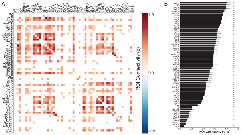
Figure 3
Whole-brain intrinsic functional connectivity
(A) Significant functional connections between brain atlas regions (N = 61 ROIs). For significant functional connections, the strength of each connection represents the Fisher transformed correlation ...
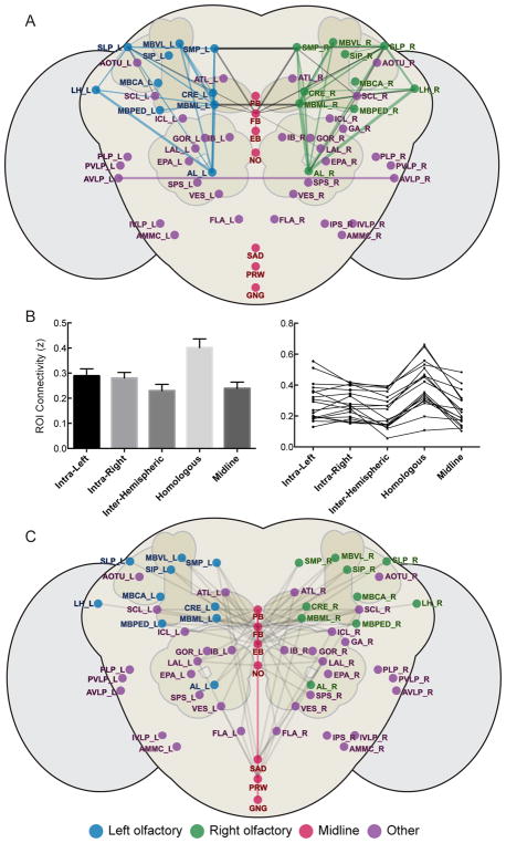
Figure 4
Organizational properties of intrinsic brain networks network in Drosophila
(A) Fly brain network with labeled atlas regions represented as circles and functional connections between them represented as lines. Atlas regions are shown over a schematized fly brain with optic lo...
Figure images are served from the NIH/NLM PubMed Central Open Access Subset or Europe PMC; copyright remains with the publishers and authors.
💬 Discussion
0 commentsNo comments yet. Be the first to start a discussion!
Leave a Comment