Abstract
Activity in striatal direct- and indirect-pathway spiny projection neurons (SPNs) is critical for proper movement. However, little is known about the spatiotemporal organization of this activity. We investigated the spatiotemporal organization of SPN ensemble activity in mice during self-paced, natural movements using microendoscopic imaging. Activity in both pathways showed predominantly local but also some long-range correlations. Using a novel approach to cluster and quantify behaviors based on continuous accelerometer and video data, we found that SPN ensembles active during specific actions were spatially closer and more correlated overall. Furthermore, similarity between different actions corresponded to the similarity between SPN ensemble patterns, irrespective of movement speed. Consistently, the accuracy of decoding behavior from SPN ensemble patterns was directly related to the dissimilarity between behavioral clusters. These results identify a predominantly local, but not spatially compact, organization of direct- and indirect-pathway SPN activity that maps action space independently of movement speed.
🔬 Techniques
💻 Software
✨ Fluorophores
🧪 Sample Preparation
🏭 Microscope Brands
🧪 Reagent Suppliers
💻 Software Details
🏷️ Research Resource Identifiers (RRIDs)
Verified research resources used in this paper:
🏛️ Research Organizations (ROR)
Affiliated research institutions:
📋 Methods
Key Resources Table REAGENT or RESOURCE SOURCE IDENTIFIER Antibodies
Rabbit anti-GFP Alexa Fluor-488 conjugate Molecular Probes Cat#A-21311; RRID: AB_221477 Bacterial and Virus Strains AAV5.CAG.Flex.GCaMP6f.WPRE.SV40 University of Pennsylvania Vector Core Cat#AV-5-PV2816 Experimental Models: Organisms/Strains Mouse: D1-Cre: Tg(Drd1a-cre)FK150Gsat/Mmucd MMRRC RRID: MMRRC_029178-UCD Mouse: D2-Cre: Tg(Drd2-cre)ER43Gsat/Mmucd MMRRC RRID: MMRRC_017268-UCD Mouse: A2a-Cre: B6.FVB(Cg)-Tg(Adora2a-cre)KG139Gsat/Mmucd MMRRC RRID: MMRRC_036158-UCD Software and Algorithms CNMF-E This paper; Pnevmatikakis et al., 2016 , Zhou et al., 2017 , Friedrich et al., 2017 N/A LBC This paper; Klaus and Plenz, 2016 N/A Unsupervised behavior classification algorithm This paper; Frey and Dueck, 2007 N/A Contact for Reagent and Resource Sharing Further information and requests for resources and reagents may be directed to and will be fulfilled by the Lead Contact, Rui Costa ( rc3031@columbia.edu ).
Experimental Model and Subject Details
All animal procedures were reviewed and performed in accordance with the Champalimaud Center for the Unknown Ethics committee guidelines and approved by the Portuguese Veterinary General Board (Direcção Geral de Veterinária, Ref. No. 0421/000/000/2014). Experimental mice were 3 to 5 month-old BAC transgenic males individually housed on a 12 hr light/dark cycle with ad libitum access to food and water. Transgenic mice expressed Cre recombinase under the control of the dopamine D1 receptor (D1-Cre, Tg(Drd1a-cre)FK150Gsat/Mmucd; MMRRC #029178-UCD) for targeting of direct-pathway SPNs, or the dopamine D2 receptor (D2-Cre, Tg(Drd2-cre)ER43Gsat/Mmucd; MMRRC #017268-UCD) or adenosine A2a receptor (A2a-Cre, B6.FVB(Cg)-Tg(Adora2a-cre)KG139Gsat/Mmucd; MMRRC #036158-UCD) for targeting of indirect-pathway SPNs. All lines have been backcrossed onto C57Bl6/J mice for at least 8 generations. Sample size is detailed in the Results or figure legends.
Show full methods section
Key Resources Table REAGENT or RESOURCE SOURCE IDENTIFIER Antibodies
Rabbit anti-GFP Alexa Fluor-488 conjugate Molecular Probes Cat#A-21311; RRID: AB_221477 Bacterial and Virus Strains AAV5.CAG.Flex.GCaMP6f.WPRE.SV40 University of Pennsylvania Vector Core Cat#AV-5-PV2816 Experimental Models: Organisms/Strains Mouse: D1-Cre: Tg(Drd1a-cre)FK150Gsat/Mmucd MMRRC RRID: MMRRC_029178-UCD Mouse: D2-Cre: Tg(Drd2-cre)ER43Gsat/Mmucd MMRRC RRID: MMRRC_017268-UCD Mouse: A2a-Cre: B6.FVB(Cg)-Tg(Adora2a-cre)KG139Gsat/Mmucd MMRRC RRID: MMRRC_036158-UCD Software and Algorithms CNMF-E This paper; Pnevmatikakis et al., 2016 , Zhou et al., 2017 , Friedrich et al., 2017 N/A LBC This paper; Klaus and Plenz, 2016 N/A Unsupervised behavior classification algorithm This paper; Frey and Dueck, 2007 N/A Contact for Reagent and Resource Sharing Further information and requests for resources and reagents may be directed to and will be fulfilled by the Lead Contact, Rui Costa ( rc3031@columbia.edu ).
Experimental Model and Subject Details
All animal procedures were reviewed and performed in accordance with the Champalimaud Center for the Unknown Ethics committee guidelines and approved by the Portuguese Veterinary General Board (Direcção Geral de Veterinária, Ref. No. 0421/000/000/2014). Experimental mice were 3 to 5 month-old BAC transgenic males individually housed on a 12 hr light/dark cycle with ad libitum access to food and water. Transgenic mice expressed Cre recombinase under the control of the dopamine D1 receptor (D1-Cre, Tg(Drd1a-cre)FK150Gsat/Mmucd; MMRRC #029178-UCD) for targeting of direct-pathway SPNs, or the dopamine D2 receptor (D2-Cre, Tg(Drd2-cre)ER43Gsat/Mmucd; MMRRC #017268-UCD) or adenosine A2a receptor (A2a-Cre, B6.FVB(Cg)-Tg(Adora2a-cre)KG139Gsat/Mmucd; MMRRC #036158-UCD) for targeting of indirect-pathway SPNs. All lines have been backcrossed onto C57Bl6/J mice for at least 8 generations. Sample size is detailed in the Results or figure legends.
Method Details Virus injection and chronic lens implantation
Surgeries were performed under sterile conditions and isoflurane (1%–3%, plus oxygen at 1-1.5 l/min) anesthesia on a stereotactic frame (David Kopf Instruments, Model 962LS). Throughout each surgery, mouse body temperature was maintained at 34°C using an animal temperature controller (ATC1000, World Precision Instruments) and afterward, each mouse was allowed to recover from the anesthesia in its homecage on a heating pad. The mouse head was shaved, cleaned with 70% alcohol and iodine, and a small incision from anterior to posterior was made on the skin to allow for aligning the head and drilling the hole for the injection site. Each animal was unilaterally injected with 300 nl of AAV5.CAG.Flex.GCaMP6f.WPRE.SV40 (University of Pennsylvania Vector Core) into the left dorsal striatum (AP: 0.5 mm, ML: 2.3 mm, DV: −2.3 mm) using a Nanojet II Injector (Drummond Scientific, USA) at a rate of 4.6 nl per pulse every 5 s. The injection pipette was left in place for 10 min post-injection before it was removed. After the injection, the skull was cleaned and the skin sealed with Vetbond tissue adhesive (3M, USA). Following the same surgical procedures, one week after viral injection, a 1-mm-diameter gradient index (GRIN) lens (Inscopix) was implanted in the left mouse striatum directly above the injection site after carefully aspirating ∼1.8-2 mm of the overlaying cortical tissue with a 30-gauge blunt needle. Care was taken to minimize bleeding. Once in place, the lens was secured to the skull using a combination of black Ortho-Jet powder and liquid acrylic resin (Lang Dental, USA) and covered with paper/tape to protect the lens surface. One week after the GRIN lens implantation, the microendoscope baseplate (Inscopix) was mounted onto the mouse head under visual guidance using the attached microscope to determine the best field of view. The imaging field of view was inspected and allowed to clear for several days prior to imaging and behavioral experiments. After completion of the behavioral experiments, mice were transcardially perfused with saline and 4% paraformaldehyde in PBS. Brains were removed for histological analysis and coronal slices were sectioned at 50 μm (Leica vibratome VT1000). Immunohistochemistry was performed for GCaMP-GFP expression by incubating the sections with a GFP antibody (GFP Tag polyclonal antibody, Alexa Fluor 488 conjugate, Molecular Probes #A-21311) diluted at 1:1000 in 0.4% Triton-PBS overnight at room temperature and counterstained with DAPI. Both placement of lens and spread of injection were confirmed using a Zeiss Lumar widefield fluorescence microscope ( Figures 1 B and S1 A).
Behavior
Mice were placed in an open field arena (39.5 × 39.5 × 17.5 cm, length × width × height) inside a sound-attenuating chamber and imaged for 10-15 min every day for 5 days during the light cycle. Behavior was recorded using an overhead-mounted video camera (Flea3, Point Grey Research) at 15-30 frames per second (fps) and a head-mounted 3-axis accelerometer sampled at 1 kHz with a Cerebus acquisition system (Blackrock Microsystems). One-photon imaging of intracellular calcium activity was acquired at 7-10 fps using an nVista microendoscope [lens: 1 mm diameter, ∼4 mm length, 0.5 numerical aperture, product number 1040; excitation: blue light-emitting diode (LED); excitation filter: 475/10 nm, ∼0.24-0.6 mW/mm 2 ; emission filter: 535/50 nm; Inscopix, Palo Alto, CA] and acquisition system with 12-bit resolution. The accelerometer was secured to the side of the microendoscope on the opposite side to the excitation LED. Mice were lightly anesthetized with isofluorane to facilitate mounting (and removal) of the microendoscope and accelerometer. Mice were allowed to wake up fully at least 15 min prior to image acquisition. Resulting calcium movies and acceleration data were analyzed as described below. Time stamps from the video camera, microendoscope and accelerometer were synchronized using the Cerebus recording system.
Calcium imaging analysis
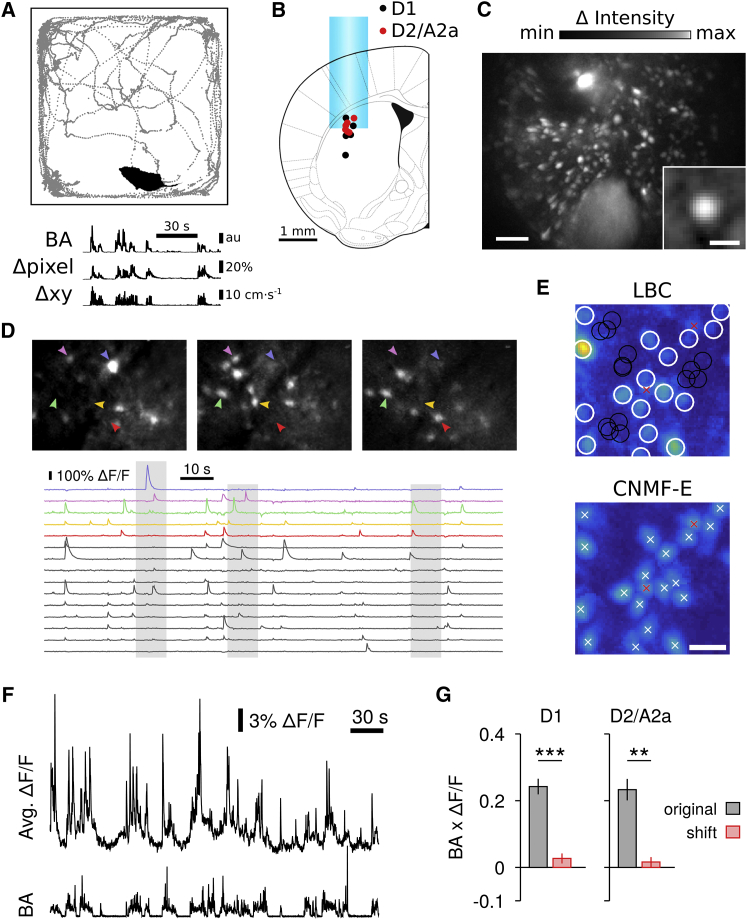
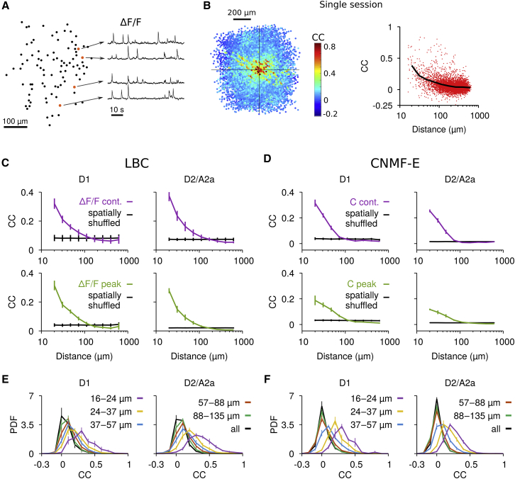
All calcium movies were initially preprocessed in Mosaic (Inscopix) for spatial binning (4 × 4 pixels) and motion correction ( Figure S1 B) and subsequently analyzed using custom MATLAB scripts. One-photon imaging is known to contain significant background signals arising from out-of-focal plane light and neuropil ( Zhou et al., 2017 ) due to the fluorescence excitation of a relatively large three-dimensional volume compared to, for example, two-photon imaging. Because out-of-focus background contains relatively low spatial frequencies ( Zhou et al., 2017 ), appropriate methods can be used to estimate background signals from the soma surrounding and correct for it. Two independent methods were employed to correct somatic calcium transients: (1) local estimation of background and baseline for fluorescence correction (LBC; Klaus and Plenz, 2016 ), and (2) a constrained non-negative matrix factorization for endoscopic data (CNMF-E; Pnevmatikakis et al., 2016 , Zhou et al., 2017 ). LBC The LBC method was based on the manual selection of somatic regions of interest (ROIs) and an automatic estimation of local background and baseline signals for fluorescence correction. A circular ROI template with diameter of 14 μm based on the half-width of the average soma shape (14.4 ± 1.0 μm, 1154 neurons from n = 10 recordings; example for single recording in Figure 1 C, inset) was used. ROIs were selected using so-called ‘activity’ images ( Figure 1 C), which were derived pixel-wise by calculating the maximum deviation over time from the average (pixel-wise) fluorescence. To allow for the identification of neurons with very low baseline fluorescence and low firing rate, ‘activity’ images were calculated for consecutive periods of 10-15 s (detailed example views shown in Figure 1 D, top) using the average fluorescence over the entire session. After manual selection of all neurons, individual background regions were determined within a 2-diameter radius around each ROI. The background region was the region with lowest average fluorescence in the ‘activity’ image with a linear penalty term for being too close to somatic ROIs. For each ROI, raw and background fluorescence (F raw and F bg , respectively) were extracted by averaging pixel intensities within the corresponding ROIs for each frame. To correct for out-of-focus background contamination, a fraction, r , of the background was subtracted from F raw ( Kerlin et al., 2010 , Pinto and Dan, 2015 ). Because blood vessels only have small contributions of neuropil signals they allow for an estimation of r, which was defined as the ratio between fluorescence in a blood vessel versus the surrounding neuropil (i.e., background). We found no difference for direct- and indirect-pathway SPN recordings (D1-Cre: 0.91 ± 0.011, D2/A2a-Cre: 0.91 ± 0.009, two-sample t test, t(13) = 0.1, p = 0.92, 2-3 recordings per subject analyzed) and used r = 0.9 for all analyses if not stated otherwise. The relative change in fluorescence was calculated as Δ F / F = F − F 0 F 0 , where F denotes the background-corrected fluorescence, F = F raw - r⋅F bg , and F 0 denotes the baseline of F fluorescence estimated from a ± 15 s sliding window. Due to the sparse activity in SPNs, F 0 was calculated from the baseline defined as the average of all values below the 80th percentile in F. The decay dynamics of intracellular calcium transients was τ decay = 299 ± 30 ms in direct-pathway SPNs and τ decay = 289 ± 20 ms in indirect-pathway SPNs in line with previous reports for GCaMP6f in pyramidal neurons of the visual cortex ( Chen et al., 2013 ). Importantly, relative increases of the intracellular, somatic calcium concentration as quantified by ΔF/F have been shown to monotonically report the number of action potentials ( Chen et al., 2013 , Cui et al., 2013 , Klaus and Plenz, 2016 ). Consequently, transient changes in ΔF/F are abolished when blocking active sodium currents using tetrodotoxin ( Cui et al., 2013 ). For some analysis, where indicated, we used time series of ΔF/F peak events to exclude possible influences of baseline fluctuations and the GCaMP6f decay dynamics. The values of the time series were set to the amplitudes of significant ΔF/F peaks at the corresponding peak times and were equal to zero otherwise. A significant ΔF/F peak event was defined by the time point and maximum value of ΔF/F during threshold crossings. The threshold was defined as mean plus three standard deviations (SDs) of the ΔF/F distribution (obtained by fitting a Gaussian function with mean and SD to the distribution of ΔF/F values individually for each neuron). Because successive (i.e., cumulative) increases in ΔF/F represent neuronal firing in successive bins, we also used, where indicated, the thresholding of the time derivative of ΔF/F, that is, the (ΔF/F(t+1)-ΔF/F(t))/Δt time series, where t represents the frame number (i.e., Δt = 1). CNMF-E Constrained non-negative matrix factorization is a recently proposed framework for simultaneously denoising, deconvolving and demixing of calcium imaging data ( Pnevmatikakis et al., 2016 ). This framework identifies the cell locations and handles spatial overlaps between neurons. CNMF-E is one of its extensions specialized for processing microendoscopic data ( Zhou et al., 2017 ). It can reliably deal with the large fluctuating background from multiple sources in the data, allowing the accurate source extraction of cellular signals. It includes four steps: (1) initialize spatial and temporal components of single neurons without the direct estimation of the background; (2) estimate the background given the estimated neurons’ spatiotemporal activity; (3) update the spatial and temporal components of all neurons while fixing the estimated background fluctuations; (4) iteratively repeat step 2 and 3. We briefly describe the algorithm used in our work, and more details can be found in the preprint of the CNMF-E paper ( Zhou et al., 2017 ). In the initialization step, we first used a mean-subtracted two-dimensional Gaussian kernel to filter the raw video data. The parameters of this kernel are selected to resemble the distribution of soma diameters (μ CNMF-E = 0, σ CNMF-E = 6.9 μm, maximum soma diameter d CNMF-E = 35 μm). Filtering the data with this kernel acts as a template matching to find all morphological shapes similar to a soma. In the filtered data, the background is approximately removed because it is almost flat within the spatial range of the kernel, and the kernel integrates to zero. In contrast, soma shapes are preserved and become more visible because they match the template shape. As a result, we can accurately extract each neuron’s calcium activity from the fluorescence at its center pixels (so-called seed pixels) in the filtered data. Furthermore, we developed a method to detect seed pixels by choosing pixels with high local correlations and signal-to-noise ratio. Given a seed pixel, we initialize one neuron by estimating its temporal activity as the temporal trace of the pixel in the filtered data. To get its spatial component, we crop a small square with the size of 2 times larger than a cell body centered at the seed pixel from the raw data. Then we estimate the background fluctuation within the cropped area as the median in each frame. For each pixel within the selected square, we assume its fluctuations are from two sources: one is the initialized neuron and the other one is the background fluctuation. Since we have the temporal traces for all these two sources, we run linear regression to get the weights for each component and the weights corresponding to the neural activity lead to our initialization of the spatial footprints. Once we have both the spatial and temporal component of this neuron, we subtract its spatiotemporal activity from the raw video data and repeat the same procedure to initialize another neuron until the specified number of neurons has been detected or no more seed pixels can be found. This greedy initialization method is able to efficiently and accurately detect almost all neurons. In the next step, we estimate the background activity for each pixel individually. For each pixel, we first choose its neighbors with a distance larger than neuron size. Accordingly, these pixels do not share the same cellular activity but they share the same sources of the background. Then we use the projection of this pixel’s temporal trace on a linear span of its neighbors’ traces as the estimated background fluctuations. Finally, we subtract this estimated background from the raw video data and update all neuronal spatial and temporal components using alternating matrix factorization ( Friedrich et al., 2017 , Pnevmatikakis et al., 2016 , Zhou et al., 2017 ). The temporal deconvolution step for denoising was used for the update of the temporal activity. The final temporal, neuronal components reported for CNMF-E were not denoised and are denoted with a capital letter C throughout the paper. Time series of significant C peak events were calculated as described for ΔF/F (see LBC above).
Analysis of ground truth data
We investigated whether LBC and CNMF-E were able to recover the underlying CC-distance relationship in simulated ground truth data ( Figures S1 C, S2D, and S2E). To simulate the strong background component in microendoscopic imaging data, we used the sum of 10 time-varying background frames with individual temporal profiles and added neuronal signals plus random noise to this image sequence. The following parameters were matched between simulated and experimental data: mean fluorescence intensity and standard deviation, average neuron diameter, number of neurons per session, neuron locations, GCaMP6f decay time constant, amplitudes of somatic fluorescence changes, and individual neuronal activity patterns obtained from the original calcium recordings (events were detected by thresholding ΔF/F > 3 SD of baseline, see description of significant ΔF/F peak events above). To obtain a flat CC-distance relationship, we randomized the neuron positions as described below in Calculation of spatially shuffled datasets . The resulting calcium movies were analyzed with LBC and CNMF-E as described above. For the LBC method, we re-applied the positions of the neuronal ROIs from the original dataset.
Calculation of CC
For the calculation of the CC between two time series x and y , we used Pearson’s correlation coefficient: C C = E [ ( x − μ x ) ( y − μ y ) ] σ x σ y , where E[·] denotes the expected operator and μ and σ denote the mean and standard deviation, respectively. Average CCs between neuronal activities were reported as the average across neuronal pairs. For the calculation of CCs between “action-related”/“other” SPNs ( Figure 3 ), see “ Definition of action-related neurons ” below. To exclude possible influences of baseline fluctuations and the GCaMP6f decay dynamics on the CC measure, we calculated, where indicated, CC on time series of significant peak events in ΔF/F (LBC) or C (CNMF-E), or their time derivatives. To determine whether average CCs were significantly larger than zero, we corrected the CC by chance-level correlations. That is, CCs obtained from significant events in the time derivative of ΔF/F were calculated and the CCs from temporally shuffled data preserving the inter-event interval distributions for each neuron were subtracted. We furthermore verified that our CC measure was not affected by the optical properties of the GRIN lens due to, for example, optical aberrations ( Figure S2 A). For the quantification of the correlation between BA and neuronal activity in Figure 1 G, ΔF/F was the average activity of all SPNs in the recording session. Time-shifted controls were obtained by randomly shifting the BA time series between ± (20-30) s. CCs for time-shifted traces were averaged over 1000 random instances per session.
Calculation of spatially shuffled datasets
Spatial shuffling of calcium activity was performed by randomizing the mapping between neuron position and activity. Specifically, for each neuron, a random neuron from the same session was selected, and the 2-dimensional positions were swapped. This approach preserved the distribution of pairwise distances between neurons as well as the precise temporal distribution of calcium events. The latter aspect is particularly relevant for continuous time series of ΔF/F (LBC) and C (CNMF-E), which contain temporal correlations due to the GCaMP6f decay dynamics that need to be preserved for the comparison to original data. We calculated 10 shuffled instances per session and used average values for further calculation. In addition, the spatial shuffling allowed us to study the influence of specific SPN ensemble configurations for the behavior decoding ( Figure 5 ) without changing the average SPN activity during each behavior. Therefore, the magnitude reduction of the correlation between behavioral similarity and percentage of correct classification ( Figures 5 B and 5C) can be attributed solely to the randomization of the spatial SPN ensemble pattern. Comparison to Barbera et al. (2016) To cluster the neuronal activity, we applied a meta-clustering approach to the neuronal data that was recently proposed by Barbera et al. (2016) . We used the same parameters as in their study. Specifically, we applied k-means clustering with k-means++ initialization to ΔF/F time series from randomly selected 30 s windows. The number of clusters was set to N where N denotes the number of neurons. The clustering was repeated 100 times per 30 s window using different k-means++ initializations. This procedure was repeated for a total of 100 30 s windows resulting in an average overlap of ∼80% between windows. A N × N co-occurrence matrix, M , was built, which contained at position i,j the number of times neuron i and neuron j were clustered together. Accordingly, M i,j = 0 if neurons i and j were never clustered together, and M i,j = 10,000 if neurons i and j were always clustered together. From the final co-occurrence matrix, meta-clusters were obtained by applying a threshold, T , and determining the largest neuronal groups. T was chosen to maximize the ratio between number of meta-clusters and number of unclustered neurons. We performed this analysis on the neuronal (i.e., soma) signals, the raw data, and the background signal obtained with CNMF-E. All signals were baseline-corrected as described in LBC . For the calculation of average intra-cluster distance and CC, only clusters with at least 5 members were used. As shown in Figures S2 H–S2J, the above meta-clustering did result in spatially extended, non-compact neuronal clusters, which was in contrast to the compact clusters reported by Barbera et al. (2016) . Because we used GCaMP6 ‘fast’ in the current study, in contrast to GCaMP6 ‘slow’ used in Barbera et al. (2016) , we verified that the spatially extended, non-compact clusters in our data were not a result of a difference in the GCaMP6 decay dynamics. To this end, we convolved continuous ΔF/F and ΔF/F peak time series with an exponential kernel with different decay time constants (up to 2 s) and found spatially extended, non-compact clusters irrespective of the chosen decay time constant (data not shown). This result suggests that the discrepancy between the current study and Barbera et al. (2016) might be due to differences in the extraction of intracellular calcium time series from raw fluorescence data. As described above, fluorescence signals obtained with one-photon calcium imaging require proper background subtraction to correct for strong out-of-focus contributions from neuropil and other sources ( Zhou et al., 2017 ) and baseline subtraction to correct for slow trends due to, for example, photobleaching. We note that the approach used by Barbera et al. to calculate relative fluorescence changes, ΔF/F, differs in two details from LBC, which previously has been shown to reliably report intracellular action potential firing ( Klaus and Plenz, 2016 ). First, Barbera et al. perform baseline subtraction on soma and background fluorescence before background-correcting the somatic fluorescence. Second, they used the minimum value of the image stack for subtraction from the raw fluorescence. This latter step, however, is not suited to remove slow trends in raw fluorescence time series and could potentially affect CC measures.
Measurement and quantification of behavior
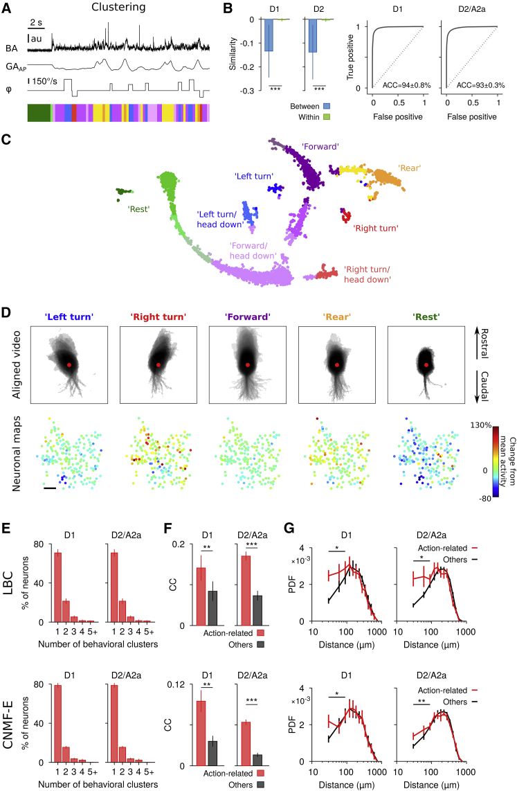
Behavior was quantified on time series of acceleration and video rotation. In the main analysis ( Figures 3 , 4 , and 5 ), we used: (i) total body acceleration to distinguish movement versus rest ( Figure 1 A), (ii) gravitational acceleration along the rostro-caudal/anterior-posterior (AP) axis to extract postural changes ( Figure S3 B), and (iii) rotational information extracted from the video to measure head and whole-body orientation ( Figures 3 A–3D). Total body acceleration was defined as B A = B A A P 2 + B A M L 2 + B A D V 2 , where BA AP/ML/DV denote the body acceleration in the anterio-posterior, mediolateral, and dorsoventral axis, respectively, with respect to the animal’s head. The individual BA components were calculated by median-filtering the raw acceleration time series and by subsequent high-pass (0.5 Hz) filtering with a fourth-order Butterworth filter. Gravitational acceleration, GA, was obtained for each axis by median and subsequent low-pass filtering (0.5 Hz cutoff, fourth-order Butterworth filter). We used GA AP to quantify postural changes (i.e., vertical head position) in the open field during resting, locomotion and rearing (regression on the GA AP and vertical head-position time series: R 2 = 0.72-0.76, p < 0.001 for n = 2 mice; Figure S3 B). Head and body rotation angle of the animal was extracted from video as relative (i.e., frame-to-frame) change in body/head axis orientation. We then converted the time series into cumulative changes of head/body rotation (positive for left rotations, negative for right rotations) to remove small rotations and noise by considering only rotations with at least ± 20°/s of cumulative change before any change in direction. The angle, φ, for each rotation was then set to the maximum relative change between the beginning (±30-60°/s) and end (i.e., change in direction) of the rotation. This step improved the detection of left and right turns using the clustering algorithm described below compared to cumulative changes in head/body rotation. An example time series of φ is shown in Figures 3 A and S3 A. Time series of all features were binned into 300 ms long, non-overlapping segments ( Wiltschko et al., 2015 ), which were used for the following clustering analysis. For each 300-ms segment and per feature, values were discretized using one or two thresholds: For BA, a single threshold was used to separate moving from resting. The threshold was the same for all subjects and was set to the average value separating the bimodal distribution of BA (visualized in logarithmic scale; Figure S3 A). For GA AP , 2 thresholds were used based on Otsu’s method ( Figure S3 A). For φ, we used 2 thresholds (±45-90°/s) separating left and right turns from straight and forward movements. The resulting histograms, that is, 3 per 300-ms segment, were individually normalized to obtain probability distributions and then used to calculate pairwise similarities between segments ( Figure S3 A). For a 600 s long recording and 300 ms long segments, this resulted in a 2000 × 2000 similarity matrix. Our measure of similarity, S , was based on the so-called “earth mover’s” (EM) distance ( Rubner et al., 2000 ): S = − ( D E M / 3 ) 2 , where D EM is the sum of the normalized EM distances for the 3 features (BA, GA AP , and φ) as defined below. The normalizations constrain the values of S to be within the range [-1,0], that is, −1 and 0 indicate the maximum dissimilarity and identity between the two probability distributions, respectively. For each single feature, the normalized EM distance between probability distributions p = ( p 1 , p 2 , … ) and q = ( q 1 , q 2 , … ) is calculated iteratively as follows: d 0 = 0 d i + 1 = ( p i + d i ) − q i , where i iterates over the number of bins of the probability distributions, that is, i = { 1,2 } for BA, and i = { 1,2,3 } for GA AP and φ. The EM distance for a single feature is then defined as E M D = ∑ i | d i | , and subsequently normalized by the number of bins minus 1. D EM is defined as the sum of the normalized EMDs. The EM-similarity, S , has a unique advantage over other measures of similarity, such as the histogram intersection similarity ( Zhang and Lu, 2003 ), or similarity based on the cross-validated Euclidean distance ( Walther et al., 2016 ). Similar to intersection and Euclidean similarity, the EM-similarity S takes into account the pairwise differences between corresponding bins in the two distributions to be compared. The unique property of S is that it also considers the distance between the bins within the distribution. For example, the probability density for the rotation φ has three bins corresponding to ‘left’, ‘straight’, and ‘right’. While intersection and Euclidean similarity attribute the same distance to ‘left’ versus ‘straight’ and ‘left’ versus ‘right’, the EM-similarity considers the distance between ‘left’ versus ‘right’ to be bigger. This makes intuitively sense because movements are generally smooth, that is, φ will not jump from ‘left’ to ‘right’ but will be ‘straight’ in between. Despite this difference, the three similarity measures (i.e., EM-similarity, intersection similarity, and cross-validated Euclidean similarity) were correlated and gave highly similar results. The obtained similarity measures ( Figure S3 A) were clustered using affinity propagation ( Frey and Dueck, 2007 ) with the preference parameter set to −0.5 (similar results were obtained over a wide range tested; the particular value was chosen to maximize the accuracy of cluster separation, see Figure 3 B, while maintaining a stable number of behavioral clusters). Using this method, we are able to generate a continuous unbiased classification of behavioral states ( Figures 3 A–3D; Movie S2 ). Based on this clustering, we finally calculated a matrix of similarities, S i , j B e h a v i o r = S ( Figure 4 A, left), using the average distribution over all 300-ms segments within behavioral clusters i and j , respectively ( i and j range from 1 to the number of behavioral clusters within the session). The analysis in Figures 4 C–4F and 5 was restricted to clusters with movement (“move”). To this end, we excluded clusters with average BA less than 2 times the threshold used for behavioral clustering (see above). See Figures S4 D and S4E for the summary of move plus rest behavioral clusters.
Visualization of behavioral similarity in two dimensions
For the visualization of behavioral time bins in two dimensions ( Figure 3 C), we used the non-linear dimensionality reduction technique t-SNE ( van der Maaten and Hinton, 2008 ). We used the matrix of pairwise EM-distances (D EM , with 5% added, uniform noise) for all behavioral histograms (i.e., 300 ms time bins) as the input for the algorithm. We verified that the Euclidean distance in the two-dimensional projection appropriately reflected the true EM-distance ( Figure S3 C). Definition of action-related neurons To determine the statistical significance of action-related increases in activity at the single-neuron level ( Figures 3 and S3 F–S3H), we applied, for each neuron and behavioral cluster, a threshold to the average ΔF/F (LBC) or C (CNMF-E), and considered the neuron to be significantly modulated if the average during the behavioral cluster crossed the 99 th percentile of shuffled data (i.e., the ‘baseline’ average during the entire recording session). The shuffled data for a given behavioral cluster was obtained by randomizing the start time stamp of each behavioral segment (i.e., preserving their durations) and calculating the average ΔF/F (LBC) and C (CNMF-E) during these randomized segments. 10,000 shuffled instances were used to calculate the ‘baseline’ average and its 99 th percentile. In Figure 3 , we restricted the analysis to neurons that showed significant positive modulations in activity (“action-related”). Figures S3 G and S3H shows quantification for SPNs with significant decrease. The calculation of pairwise measures (i.e., CC and inter-neuron distance; Figures 3 E–3G and S3 H) for “action-related” and “other” neurons was done for each behavioral cluster and final values were averaged across behavioral clusters within the same recording session. Thus, neurons considered “other” for one particular behavioral cluster, could be “action-related” for another behavioral cluster. CCs were calculated using the entire time series (ΔF/F for LBC; C for CNMF-E). We note that for the analysis at the SPN ensemble level ( Figures 4 and 5 ), we included all neurons imaged during the recording session.
Quantification of neuronal similarity
For each behavioral cluster, we extracted for all neurons, the time-averaged calcium activities, ΔF/F and C (for LBC and CNMF-E, respectively) during the cluster. This resulted in an n-dimensional vector, x , for each behavioral cluster that represents the SPN ensemble patterns during that behavior (n denotes the number of all recorded neurons during the imaging session). To quantify the similarity between those SPN ensemble patterns ( Figure 4 ), we used a similarity measure based on the cross-validated Euclidean distance ( Walther et al., 2016 ). To this end, we divided calcium activities into odd and even image frame numbers to obtain unbiased estimates of the similarity between SPN ensemble patterns ( Figure 4 A, right): S i , j N e u r o n a l = − ( x i − x j ) o d d ( x i − x j ) e v e n T , where x i and x j denote the SPN ensemble vectors for behavioral clusters i and j , respectively ( i and j range from 1 to the number of behavioral clusters within the session). We note that dividing the dataset into first and second half for the above calculation of cross-validated measures, or similarity based on crosscorrelation between the SPN ensemble vectors, gave similar results. Because changes in the average SPN population activity (as evident in Figures 1 F, 1G, and 3 D) could contribute to the estimate of the Euclidean similarity between SPN ensemble patterns, we normalized the ensemble vector x to have a Euclidean norm equal to unity ( Figure 4 ; similar results were obtained without normalization or normalization of the mean, i.e., average across SPNs equal to one). To quantify the relationship between behavioral and neuronal similarity ( Figures 4 B–4F), we used the Spearman correlation coefficient ρ. ρ and corresponding p -values were calculated using MATLAB’s corr function. Behavioral clusters with less than 10 occurrences were excluded from the analysis. Furthermore, sessions with less than four data points for the calculation of ρ were excluded from the calculation of averages. To test the influence of movement versus resting on the relationship between behavioral and neuronal similarity, we performed two control measures. First, the analysis was, in addition to all clusters (moving and resting, Figure 4 B, gray), performed only on clusters with strong movement ( Figure 4 B, red; Figures 4 C–4F; see Measurement and quantification of behavior for the definition of the threshold separating moving from resting). Second, behavioral similarity was, in addition to the full features set (BA, GA AP , φ), performed only on the similarity in BA (i.e., the cross-validated difference in average BA during the behavioral clusters) ( Figures 4 D and 4F), or movement speed (i.e., cross-validated difference in average video pixel change during the behavioral clusters). For spatially shuffled control measures, the mapping between neuron position and neuronal activity (ΔF/F for LBC; C for CNMF-E) was randomized for each session and each behavioral cluster (see Calculation of spatially shuffled datasets ). Decoding of behavior from SPN ensemble activities For the decoding analysis of behaviors from SPN ensemble activities, we used a linear support vector machine (SVM) for binary classification. The aim of the decoding was to predict the behavioral cluster membership obtained with affinity propagation (see above) based on the SPN ensemble activity at the timescale of the behavioral segments. Many behavioral segments were as short as 300 ms (the bin size for the behavioral clustering) but could range, in multiples of 300 ms, to many seconds ( Figure S4 C). For each behavioral segment obtained with our behavioral clustering approach, we first determined the corresponding SPN calcium activities, and averaged them during that segment. This resulted in n-dimensional vectors representing the SPN ensemble patterns, where n is equal to the number of all recorded neurons during the imaging session. The vectors representing the SPN ensemble patterns and the information about which behavioral cluster they belong to where then used to train and evaluate the SVM. Specifically, for each pair of behavioral clusters, a random set of 60% of the data was used for training the SVM, while the remaining data was used for evaluating the decoding accuracy quantified as the percentage of correct classifications (“percentage correct”; Figure 5 ). We averaged the “percentage correct” over 10 random training/evaluation datasets to obtain more reliable estimates. To account for sample number differences between behavioral clusters i and j and a possible classification bias, the percentage correct was calculated as the average between the percentage correct for behavioral cluster i and percentage correct for behavioral cluster j . The decoding analysis gave similar results for non-normalized and normalized SPN ensemble activity. Results in Figure 5 are shown for non-normalized SPN ensemble activity. The spatial shuffling (see above) in Figure 5 was done for each behavioral segment, thus preserving the average SPN activity within each behavioral cluster. This allowed attributing differences in the behavior decoding between original and spatially shuffled data solely to the precise configuration of the original SPN ensemble patterns and not the average SPN activity. For the quantification of the relationship between “behavioral similarity” and “percentage correct” in Figure 5 , we used the Spearman correlation coefficient ρ and followed the same approach as described in Quantification of neuronal similarity for Figure 4 . Quantification and Statistical Analysis Mean ± standard error of the mean (SEM) was used to report statistics if not indicated otherwise. For all within-subject quantifications, we calculated the average across all 5 recording sessions. Statistical tests used and the sample size for each analysis is listed in the Results or figure legends. Both parametric and non-parametric tests were used wherever appropriate and are detailed in the Results and Table S1 . Hypothesis testing was done at a significance level of α = 0.05. No statistical methods were used to pre-determine sample size. Where required, datasets were tested for normality using the Lilliefors test. All analysis and statistical tests were performed in MATLAB (MathWorks). Animals were excluded prior to the collection of experimental data based on imaging quality due to movement artifact, a lack of cells, or a bad focal plane.
Experimental Model and Subject Details
All animal procedures were reviewed and performed in accordance with the Champalimaud Center for the Unknown Ethics committee guidelines and approved by the Portuguese Veterinary General Board (Direcção Geral de Veterinária, Ref. No. 0421/000/000/2014). Experimental mice were 3 to 5 month-old BAC transgenic males individually housed on a 12 hr light/dark cycle with ad libitum access to food and water. Transgenic mice expressed Cre recombinase under the control of the dopamine D1 receptor (D1-Cre, Tg(Drd1a-cre)FK150Gsat/Mmucd; MMRRC #029178-UCD) for targeting of direct-pathway SPNs, or the dopamine D2 receptor (D2-Cre, Tg(Drd2-cre)ER43Gsat/Mmucd; MMRRC #017268-UCD) or adenosine A2a receptor (A2a-Cre, B6.FVB(Cg)-Tg(Adora2a-cre)KG139Gsat/Mmucd; MMRRC #036158-UCD) for targeting of indirect-pathway SPNs. All lines have been backcrossed onto C57Bl6/J mice for at least 8 generations. Sample size is detailed in the Results or figure legends.
Method Details Virus injection and chronic lens implantation
Surgeries were performed under sterile conditions and isoflurane (1%–3%, plus oxygen at 1-1.5 l/min) anesthesia on a stereotactic frame (David Kopf Instruments, Model 962LS). Throughout each surgery, mouse body temperature was maintained at 34°C using an animal temperature controller (ATC1000, World Precision Instruments) and afterward, each mouse was allowed to recover from the anesthesia in its homecage on a heating pad. The mouse head was shaved, cleaned with 70% alcohol and iodine, and a small incision from anterior to posterior was made on the skin to allow for aligning the head and drilling the hole for the injection site. Each animal was unilaterally injected with 300 nl of AAV5.CAG.Flex.GCaMP6f.WPRE.SV40 (University of Pennsylvania Vector Core) into the left dorsal striatum (AP: 0.5 mm, ML: 2.3 mm, DV: −2.3 mm) using a Nanojet II Injector (Drummond Scientific, USA) at a rate of 4.6 nl per pulse every 5 s. The injection pipette was left in place for 10 min post-injection before it was removed. After the injection, the skull was cleaned and the skin sealed with Vetbond tissue adhesive (3M, USA). Following the same surgical procedures, one week after viral injection, a 1-mm-diameter gradient index (GRIN) lens (Inscopix) was implanted in the left mouse striatum directly above the injection site after carefully aspirating ∼1.8-2 mm of the overlaying cortical tissue with a 30-gauge blunt needle. Care was taken to minimize bleeding. Once in place, the lens was secured to the skull using a combination of black Ortho-Jet powder and liquid acrylic resin (Lang Dental, USA) and covered with paper/tape to protect the lens surface. One week after the GRIN lens implantation, the microendoscope baseplate (Inscopix) was mounted onto the mouse head under visual guidance using the attached microscope to determine the best field of view. The imaging field of view was inspected and allowed to clear for several days prior to imaging and behavioral experiments. After completion of the behavioral experiments, mice were transcardially perfused with saline and 4% paraformaldehyde in PBS. Brains were removed for histological analysis and coronal slices were sectioned at 50 μm (Leica vibratome VT1000). Immunohistochemistry was performed for GCaMP-GFP expression by incubating the sections with a GFP antibody (GFP Tag polyclonal antibody, Alexa Fluor 488 conjugate, Molecular Probes #A-21311) diluted at 1:1000 in 0.4% Triton-PBS overnight at room temperature and counterstained with DAPI. Both placement of lens and spread of injection were confirmed using a Zeiss Lumar widefield fluorescence microscope ( Figures 1 B and S1 A).
Behavior
Mice were placed in an open field arena (39.5 × 39.5 × 17.5 cm, length × width × height) inside a sound-attenuating chamber and imaged for 10-15 min every day for 5 days during the light cycle. Behavior was recorded using an overhead-mounted video camera (Flea3, Point Grey Research) at 15-30 frames per second (fps) and a head-mounted 3-axis accelerometer sampled at 1 kHz with a Cerebus acquisition system (Blackrock Microsystems). One-photon imaging of intracellular calcium activity was acquired at 7-10 fps using an nVista microendoscope [lens: 1 mm diameter, ∼4 mm length, 0.5 numerical aperture, product number 1040; excitation: blue light-emitting diode (LED); excitation filter: 475/10 nm, ∼0.24-0.6 mW/mm 2 ; emission filter: 535/50 nm; Inscopix, Palo Alto, CA] and acquisition system with 12-bit resolution. The accelerometer was secured to the side of the microendoscope on the opposite side to the excitation LED. Mice were lightly anesthetized with isofluorane to facilitate mounting (and removal) of the microendoscope and accelerometer. Mice were allowed to wake up fully at least 15 min prior to image acquisition. Resulting calcium movies and acceleration data were analyzed as described below. Time stamps from the video camera, microendoscope and accelerometer were synchronized using the Cerebus recording system.
Calcium imaging analysis
All calcium movies were initially preprocessed in Mosaic (Inscopix) for spatial binning (4 × 4 pixels) and motion correction ( Figure S1 B) and subsequently analyzed using custom MATLAB scripts. One-photon imaging is known to contain significant background signals arising from out-of-focal plane light and neuropil ( Zhou et al., 2017 ) due to the fluorescence excitation of a relatively large three-dimensional volume compared to, for example, two-photon imaging. Because out-of-focus background contains relatively low spatial frequencies ( Zhou et al., 2017 ), appropriate methods can be used to estimate background signals from the soma surrounding and correct for it. Two independent methods were employed to correct somatic calcium transients: (1) local estimation of background and baseline for fluorescence correction (LBC; Klaus and Plenz, 2016 ), and (2) a constrained non-negative matrix factorization for endoscopic data (CNMF-E; Pnevmatikakis et al., 2016 , Zhou et al., 2017 ). LBC The LBC method was based on the manual selection of somatic regions of interest (ROIs) and an automatic estimation of local background and baseline signals for fluorescence correction. A circular ROI template with diameter of 14 μm based on the half-width of the average soma shape (14.4 ± 1.0 μm, 1154 neurons from n = 10 recordings; example for single recording in Figure 1 C, inset) was used. ROIs were selected using so-called ‘activity’ images ( Figure 1 C), which were derived pixel-wise by calculating the maximum deviation over time from the average (pixel-wise) fluorescence. To allow for the identification of neurons with very low baseline fluorescence and low firing rate, ‘activity’ images were calculated for consecutive periods of 10-15 s (detailed example views shown in Figure 1 D, top) using the average fluorescence over the entire session. After manual selection of all neurons, individual background regions were determined within a 2-diameter radius around each ROI. The background region was the region with lowest average fluorescence in the ‘activity’ image with a linear penalty term for being too close to somatic ROIs. For each ROI, raw and background fluorescence (F raw and F bg , respectively) were extracted by averaging pixel intensities within the corresponding ROIs for each frame. To correct for out-of-focus background contamination, a fraction, r , of the background was subtracted from F raw ( Kerlin et al., 2010 , Pinto and Dan, 2015 ). Because blood vessels only have small contributions of neuropil signals they allow for an estimation of r, which was defined as the ratio between fluorescence in a blood vessel versus the surrounding neuropil (i.e., background). We found no difference for direct- and indirect-pathway SPN recordings (D1-Cre: 0.91 ± 0.011, D2/A2a-Cre: 0.91 ± 0.009, two-sample t test, t(13) = 0.1, p = 0.92, 2-3 recordings per subject analyzed) and used r = 0.9 for all analyses if not stated otherwise. The relative change in fluorescence was calculated as Δ F / F = F − F 0 F 0 , where F denotes the background-corrected fluorescence, F = F raw - r⋅F bg , and F 0 denotes the baseline of F fluorescence estimated from a ± 15 s sliding window. Due to the sparse activity in SPNs, F 0 was calculated from the baseline defined as the average of all values below the 80th percentile in F. The decay dynamics of intracellular calcium transients was τ decay = 299 ± 30 ms in direct-pathway SPNs and τ decay = 289 ± 20 ms in indirect-pathway SPNs in line with previous reports for GCaMP6f in pyramidal neurons of the visual cortex ( Chen et al., 2013 ). Importantly, relative increases of the intracellular, somatic calcium concentration as quantified by ΔF/F have been shown to monotonically report the number of action potentials ( Chen et al., 2013 , Cui et al., 2013 , Klaus and Plenz, 2016 ). Consequently, transient changes in ΔF/F are abolished when blocking active sodium currents using tetrodotoxin ( Cui et al., 2013 ). For some analysis, where indicated, we used time series of ΔF/F peak events to exclude possible influences of baseline fluctuations and the GCaMP6f decay dynamics. The values of the time series were set to the amplitudes of significant ΔF/F peaks at the corresponding peak times and were equal to zero otherwise. A significant ΔF/F peak event was defined by the time point and maximum value of ΔF/F during threshold crossings. The threshold was defined as mean plus three standard deviations (SDs) of the ΔF/F distribution (obtained by fitting a Gaussian function with mean and SD to the distribution of ΔF/F values individually for each neuron). Because successive (i.e., cumulative) increases in ΔF/F represent neuronal firing in successive bins, we also used, where indicated, the thresholding of the time derivative of ΔF/F, that is, the (ΔF/F(t+1)-ΔF/F(t))/Δt time series, where t represents the frame number (i.e., Δt = 1). CNMF-E Constrained non-negative matrix factorization is a recently proposed framework for simultaneously denoising, deconvolving and demixing of calcium imaging data ( Pnevmatikakis et al., 2016 ). This framework identifies the cell locations and handles spatial overlaps between neurons. CNMF-E is one of its extensions specialized for processing microendoscopic data ( Zhou et al., 2017 ). It can reliably deal with the large fluctuating background from multiple sources in the data, allowing the accurate source extraction of cellular signals. It includes four steps: (1) initialize spatial and temporal components of single neurons without the direct estimation of the background; (2) estimate the background given the estimated neurons’ spatiotemporal activity; (3) update the spatial and temporal components of all neurons while fixing the estimated background fluctuations; (4) iteratively repeat step 2 and 3. We briefly describe the algorithm used in our work, and more details can be found in the preprint of the CNMF-E paper ( Zhou et al., 2017 ). In the initialization step, we first used a mean-subtracted two-dimensional Gaussian kernel to filter the raw video data. The parameters of this kernel are selected to resemble the distribution of soma diameters (μ CNMF-E = 0, σ CNMF-E = 6.9 μm, maximum soma diameter d CNMF-E = 35 μm). Filtering the data with this kernel acts as a template matching to find all morphological shapes similar to a soma. In the filtered data, the background is approximately removed because it is almost flat within the spatial range of the kernel, and the kernel integrates to zero. In contrast, soma shapes are preserved and become more visible because they match the template shape. As a result, we can accurately extract each neuron’s calcium activity from the fluorescence at its center pixels (so-called seed pixels) in the filtered data. Furthermore, we developed a method to detect seed pixels by choosing pixels with high local correlations and signal-to-noise ratio. Given a seed pixel, we initialize one neuron by estimating its temporal activity as the temporal trace of the pixel in the filtered data. To get its spatial component, we crop a small square with the size of 2 times larger than a cell body centered at the seed pixel from the raw data. Then we estimate the background fluctuation within the cropped area as the median in each frame. For each pixel within the selected square, we assume its fluctuations are from two sources: one is the initialized neuron and the other one is the background fluctuation. Since we have the temporal traces for all these two sources, we run linear regression to get the weights for each component and the weights corresponding to the neural activity lead to our initialization of the spatial footprints. Once we have both the spatial and temporal component of this neuron, we subtract its spatiotemporal activity from the raw video data and repeat the same procedure to initialize another neuron until the specified number of neurons has been detected or no more seed pixels can be found. This greedy initialization method is able to efficiently and accurately detect almost all neurons. In the next step, we estimate the background activity for each pixel individually. For each pixel, we first choose its neighbors with a distance larger than neuron size. Accordingly, these pixels do not share the same cellular activity but they share the same sources of the background. Then we use the projection of this pixel’s temporal trace on a linear span of its neighbors’ traces as the estimated background fluctuations. Finally, we subtract this estimated background from the raw video data and update all neuronal spatial and temporal components using alternating matrix factorization ( Friedrich et al., 2017 , Pnevmatikakis et al., 2016 , Zhou et al., 2017 ). The temporal deconvolution step for denoising was used for the update of the temporal activity. The final temporal, neuronal components reported for CNMF-E were not denoised and are denoted with a capital letter C throughout the paper. Time series of significant C peak events were calculated as described for ΔF/F (see LBC above).
Analysis of ground truth data
We investigated whether LBC and CNMF-E were able to recover the underlying CC-distance relationship in simulated ground truth data ( Figures S1 C, S2D, and S2E). To simulate the strong background component in microendoscopic imaging data, we used the sum of 10 time-varying background frames with individual temporal profiles and added neuronal signals plus random noise to this image sequence. The following parameters were matched between simulated and experimental data: mean fluorescence intensity and standard deviation, average neuron diameter, number of neurons per session, neuron locations, GCaMP6f decay time constant, amplitudes of somatic fluorescence changes, and individual neuronal activity patterns obtained from the original calcium recordings (events were detected by thresholding ΔF/F > 3 SD of baseline, see description of significant ΔF/F peak events above). To obtain a flat CC-distance relationship, we randomized the neuron positions as described below in Calculation of spatially shuffled datasets . The resulting calcium movies were analyzed with LBC and CNMF-E as described above. For the LBC method, we re-applied the positions of the neuronal ROIs from the original dataset.
Calculation of CC
For the calculation of the CC between two time series x and y , we used Pearson’s correlation coefficient: C C = E [ ( x − μ x ) ( y − μ y ) ] σ x σ y , where E[·] denotes the expected operator and μ and σ denote the mean and standard deviation, respectively. Average CCs between neuronal activities were reported as the average across neuronal pairs. For the calculation of CCs between “action-related”/“other” SPNs ( Figure 3 ), see “ Definition of action-related neurons ” below. To exclude possible influences of baseline fluctuations and the GCaMP6f decay dynamics on the CC measure, we calculated, where indicated, CC on time series of significant peak events in ΔF/F (LBC) or C (CNMF-E), or their time derivatives. To determine whether average CCs were significantly larger than zero, we corrected the CC by chance-level correlations. That is, CCs obtained from significant events in the time derivative of ΔF/F were calculated and the CCs from temporally shuffled data preserving the inter-event interval distributions for each neuron were subtracted. We furthermore verified that our CC measure was not affected by the optical properties of the GRIN lens due to, for example, optical aberrations ( Figure S2 A). For the quantification of the correlation between BA and neuronal activity in Figure 1 G, ΔF/F was the average activity of all SPNs in the recording session. Time-shifted controls were obtained by randomly shifting the BA time series between ± (20-30) s. CCs for time-shifted traces were averaged over 1000 random instances per session.
Calculation of spatially shuffled datasets
Spatial shuffling of calcium activity was performed by randomizing the mapping between neuron position and activity. Specifically, for each neuron, a random neuron from the same session was selected, and the 2-dimensional positions were swapped. This approach preserved the distribution of pairwise distances between neurons as well as the precise temporal distribution of calcium events. The latter aspect is particularly relevant for continuous time series of ΔF/F (LBC) and C (CNMF-E), which contain temporal correlations due to the GCaMP6f decay dynamics that need to be preserved for the comparison to original data. We calculated 10 shuffled instances per session and used average values for further calculation. In addition, the spatial shuffling allowed us to study the influence of specific SPN ensemble configurations for the behavior decoding ( Figure 5 ) without changing the average SPN activity during each behavior. Therefore, the magnitude reduction of the correlation between behavioral similarity and percentage of correct classification ( Figures 5 B and 5C) can be attributed solely to the randomization of the spatial SPN ensemble pattern. Comparison to Barbera et al. (2016) To cluster the neuronal activity, we applied a meta-clustering approach to the neuronal data that was recently proposed by Barbera et al. (2016) . We used the same parameters as in their study. Specifically, we applied k-means clustering with k-means++ initialization to ΔF/F time series from randomly selected 30 s windows. The number of clusters was set to N where N denotes the number of neurons. The clustering was repeated 100 times per 30 s window using different k-means++ initializations. This procedure was repeated for a total of 100 30 s windows resulting in an average overlap of ∼80% between windows. A N × N co-occurrence matrix, M , was built, which contained at position i,j the number of times neuron i and neuron j were clustered together. Accordingly, M i,j = 0 if neurons i and j were never clustered together, and M i,j = 10,000 if neurons i and j were always clustered together. From the final co-occurrence matrix, meta-clusters were obtained by applying a threshold, T , and determining the largest neuronal groups. T was chosen to maximize the ratio between number of meta-clusters and number of unclustered neurons. We performed this analysis on the neuronal (i.e., soma) signals, the raw data, and the background signal obtained with CNMF-E. All signals were baseline-corrected as described in LBC . For the calculation of average intra-cluster distance and CC, only clusters with at least 5 members were used. As shown in Figures S2 H–S2J, the above meta-clustering did result in spatially extended, non-compact neuronal clusters, which was in contrast to the compact clusters reported by Barbera et al. (2016) . Because we used GCaMP6 ‘fast’ in the current study, in contrast to GCaMP6 ‘slow’ used in Barbera et al. (2016) , we verified that the spatially extended, non-compact clusters in our data were not a result of a difference in the GCaMP6 decay dynamics. To this end, we convolved continuous ΔF/F and ΔF/F peak time series with an exponential kernel with different decay time constants (up to 2 s) and found spatially extended, non-compact clusters irrespective of the chosen decay time constant (data not shown). This result suggests that the discrepancy between the current study and Barbera et al. (2016) might be due to differences in the extraction of intracellular calcium time series from raw fluorescence data. As described above, fluorescence signals obtained with one-photon calcium imaging require proper background subtraction to correct for strong out-of-focus contributions from neuropil and other sources ( Zhou et al., 2017 ) and baseline subtraction to correct for slow trends due to, for example, photobleaching. We note that the approach used by Barbera et al. to calculate relative fluorescence changes, ΔF/F, differs in two details from LBC, which previously has been shown to reliably report intracellular action potential firing ( Klaus and Plenz, 2016 ). First, Barbera et al. perform baseline subtraction on soma and background fluorescence before background-correcting the somatic fluorescence. Second, they used the minimum value of the image stack for subtraction from the raw fluorescence. This latter step, however, is not suited to remove slow trends in raw fluorescence time series and could potentially affect CC measures.
Measurement and quantification of behavior
Behavior was quantified on time series of acceleration and video rotation. In the main analysis ( Figures 3 , 4 , and 5 ), we used: (i) total body acceleration to distinguish movement versus rest ( Figure 1 A), (ii) gravitational acceleration along the rostro-caudal/anterior-posterior (AP) axis to extract postural changes ( Figure S3 B), and (iii) rotational information extracted from the video to measure head and whole-body orientation ( Figures 3 A–3D). Total body acceleration was defined as B A = B A A P 2 + B A M L 2 + B A D V 2 , where BA AP/ML/DV denote the body acceleration in the anterio-posterior, mediolateral, and dorsoventral axis, respectively, with respect to the animal’s head. The individual BA components were calculated by median-filtering the raw acceleration time series and by subsequent high-pass (0.5 Hz) filtering with a fourth-order Butterworth filter. Gravitational acceleration, GA, was obtained for each axis by median and subsequent low-pass filtering (0.5 Hz cutoff, fourth-order Butterworth filter). We used GA AP to quantify postural changes (i.e., vertical head position) in the open field during resting, locomotion and rearing (regression on the GA AP and vertical head-position time series: R 2 = 0.72-0.76, p < 0.001 for n = 2 mice; Figure S3 B). Head and body rotation angle of the animal was extracted from video as relative (i.e., frame-to-frame) change in body/head axis orientation. We then converted the time series into cumulative changes of head/body rotation (positive for left rotations, negative for right rotations) to remove small rotations and noise by considering only rotations with at least ± 20°/s of cumulative change before any change in direction. The angle, φ, for each rotation was then set to the maximum relative change between the beginning (±30-60°/s) and end (i.e., change in direction) of the rotation. This step improved the detection of left and right turns using the clustering algorithm described below compared to cumulative changes in head/body rotation. An example time series of φ is shown in Figures 3 A and S3 A. Time series of all features were binned into 300 ms long, non-overlapping segments ( Wiltschko et al., 2015 ), which were used for the following clustering analysis. For each 300-ms segment and per feature, values were discretized using one or two thresholds: For BA, a single threshold was used to separate moving from resting. The threshold was the same for all subjects and was set to the average value separating the bimodal distribution of BA (visualized in logarithmic scale; Figure S3 A). For GA AP , 2 thresholds were used based on Otsu’s method ( Figure S3 A). For φ, we used 2 thresholds (±45-90°/s) separating left and right turns from straight and forward movements. The resulting histograms, that is, 3 per 300-ms segment, were individually normalized to obtain probability distributions and then used to calculate pairwise similarities between segments ( Figure S3 A). For a 600 s long recording and 300 ms long segments, this resulted in a 2000 × 2000 similarity matrix. Our measure of similarity, S , was based on the so-called “earth mover’s” (EM) distance ( Rubner et al., 2000 ): S = − ( D E M / 3 ) 2 , where D EM is the sum of the normalized EM distances for the 3 features (BA, GA AP , and φ) as defined below. The normalizations constrain the values of S to be within the range [-1,0], that is, −1 and 0 indicate the maximum dissimilarity and identity between the two probability distributions, respectively. For each single feature, the normalized EM distance between probability distributions p = ( p 1 , p 2 , … ) and q = ( q 1 , q 2 , … ) is calculated iteratively as follows: d 0 = 0 d i + 1 = ( p i + d i ) − q i , where i iterates over the number of bins of the probability distributions, that is, i = { 1,2 } for BA, and i = { 1,2,3 } for GA AP and φ. The EM distance for a single feature is then defined as E M D = ∑ i | d i | , and subsequently normalized by the number of bins minus 1. D EM is defined as the sum of the normalized EMDs. The EM-similarity, S , has a unique advantage over other measures of similarity, such as the histogram intersection similarity ( Zhang and Lu, 2003 ), or similarity based on the cross-validated Euclidean distance ( Walther et al., 2016 ). Similar to intersection and Euclidean similarity, the EM-similarity S takes into account the pairwise differences between corresponding bins in the two distributions to be compared. The unique property of S is that it also considers the distance between the bins within the distribution. For example, the probability density for the rotation φ has three bins corresponding to ‘left’, ‘straight’, and ‘right’. While intersection and Euclidean similarity attribute the same distance to ‘left’ versus ‘straight’ and ‘left’ versus ‘right’, the EM-similarity considers the distance between ‘left’ versus ‘right’ to be bigger. This makes intuitively sense because movements are generally smooth, that is, φ will not jump from ‘left’ to ‘right’ but will be ‘straight’ in between. Despite this difference, the three similarity measures (i.e., EM-similarity, intersection similarity, and cross-validated Euclidean similarity) were correlated and gave highly similar results. The obtained similarity measures ( Figure S3 A) were clustered using affinity propagation ( Frey and Dueck, 2007 ) with the preference parameter set to −0.5 (similar results were obtained over a wide range tested; the particular value was chosen to maximize the accuracy of cluster separation, see Figure 3 B, while maintaining a stable number of behavioral clusters). Using this method, we are able to generate a continuous unbiased classification of behavioral states ( Figures 3 A–3D; Movie S2 ). Based on this clustering, we finally calculated a matrix of similarities, S i , j B e h a v i o r = S ( Figure 4 A, left), using the average distribution over all 300-ms segments within behavioral clusters i and j , respectively ( i and j range from 1 to the number of behavioral clusters within the session). The analysis in Figures 4 C–4F and 5 was restricted to clusters with movement (“move”). To this end, we excluded clusters with average BA less than 2 times the threshold used for behavioral clustering (see above). See Figures S4 D and S4E for the summary of move plus rest behavioral clusters.
Visualization of behavioral similarity in two dimensions
For the visualization of behavioral time bins in two dimensions ( Figure 3 C), we used the non-linear dimensionality reduction technique t-SNE ( van der Maaten and Hinton, 2008 ). We used the matrix of pairwise EM-distances (D EM , with 5% added, uniform noise) for all behavioral histograms (i.e., 300 ms time bins) as the input for the algorithm. We verified that the Euclidean distance in the two-dimensional projection appropriately reflected the true EM-distance ( Figure S3 C). Definition of action-related neurons To determine the statistical significance of action-related increases in activity at the single-neuron level ( Figures 3 and S3 F–S3H), we applied, for each neuron and behavioral cluster, a threshold to the average ΔF/F (LBC) or C (CNMF-E), and considered the neuron to be significantly modulated if the average during the behavioral cluster crossed the 99 th percentile of shuffled data (i.e., the ‘baseline’ average during the entire recording session). The shuffled data for a given behavioral cluster was obtained by randomizing the start time stamp of each behavioral segment (i.e., preserving their durations) and calculating the average ΔF/F (LBC) and C (CNMF-E) during these randomized segments. 10,000 shuffled instances were used to calculate the ‘baseline’ average and its 99 th percentile. In Figure 3 , we restricted the analysis to neurons that showed significant positive modulations in activity (“action-related”). Figures S3 G and S3H shows quantification for SPNs with significant decrease. The calculation of pairwise measures (i.e., CC and inter-neuron distance; Figures 3 E–3G and S3 H) for “action-related” and “other” neurons was done for each behavioral cluster and final values were averaged across behavioral clusters within the same recording session. Thus, neurons considered “other” for one particular behavioral cluster, could be “action-related” for another behavioral cluster. CCs were calculated using the entire time series (ΔF/F for LBC; C for CNMF-E). We note that for the analysis at the SPN ensemble level ( Figures 4 and 5 ), we included all neurons imaged during the recording session.
Quantification of neuronal similarity
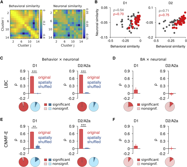
For each behavioral cluster, we extracted for all neurons, the time-averaged calcium activities, ΔF/F and C (for LBC and CNMF-E, respectively) during the cluster. This resulted in an n-dimensional vector, x , for each behavioral cluster that represents the SPN ensemble patterns during that behavior (n denotes the number of all recorded neurons during the imaging session). To quantify the similarity between those SPN ensemble patterns ( Figure 4 ), we used a similarity measure based on the cross-validated Euclidean distance ( Walther et al., 2016 ). To this end, we divided calcium activities into odd and even image frame numbers to obtain unbiased estimates of the similarity between SPN ensemble patterns ( Figure 4 A, right): S i , j N e u r o n a l = − ( x i − x j ) o d d ( x i − x j ) e v e n T , where x i and x j denote the SPN ensemble vectors for behavioral clusters i and j , respectively ( i and j range from 1 to the number of behavioral clusters within the session). We note that dividing the dataset into first and second half for the above calculation of cross-validated measures, or similarity based on crosscorrelation between the SPN ensemble vectors, gave similar results. Because changes in the average SPN population activity (as evident in Figures 1 F, 1G, and 3 D) could contribute to the estimate of the Euclidean similarity between SPN ensemble patterns, we normalized the ensemble vector x to have a Euclidean norm equal to unity ( Figure 4 ; similar results were obtained without normalization or normalization of the mean, i.e., average across SPNs equal to one). To quantify the relationship between behavioral and neuronal similarity ( Figures 4 B–4F), we used the Spearman correlation coefficient ρ. ρ and corresponding p -values were calculated using MATLAB’s corr function. Behavioral clusters with less than 10 occurrences were excluded from the analysis. Furthermore, sessions with less than four data points for the calculation of ρ were excluded from the calculation of averages. To test the influence of movement versus resting on the relationship between behavioral and neuronal similarity, we performed two control measures. First, the analysis was, in addition to all clusters (moving and resting, Figure 4 B, gray), performed only on clusters with strong movement ( Figure 4 B, red; Figures 4 C–4F; see Measurement and quantification of behavior for the definition of the threshold separating moving from resting). Second, behavioral similarity was, in addition to the full features set (BA, GA AP , φ), performed only on the similarity in BA (i.e., the cross-validated difference in average BA during the behavioral clusters) ( Figures 4 D and 4F), or movement speed (i.e., cross-validated difference in average video pixel change during the behavioral clusters). For spatially shuffled control measures, the mapping between neuron position and neuronal activity (ΔF/F for LBC; C for CNMF-E) was randomized for each session and each behavioral cluster (see Calculation of spatially shuffled datasets ). Decoding of behavior from SPN ensemble activities For the decoding analysis of behaviors from SPN ensemble activities, we used a linear support vector machine (SVM) for binary classification. The aim of the decoding was to predict the behavioral cluster membership obtained with affinity propagation (see above) based on the SPN ensemble activity at the timescale of the behavioral segments. Many behavioral segments were as short as 300 ms (the bin size for the behavioral clustering) but could range, in multiples of 300 ms, to many seconds ( Figure S4 C). For each behavioral segment obtained with our behavioral clustering approach, we first determined the corresponding SPN calcium activities, and averaged them during that segment. This resulted in n-dimensional vectors representing the SPN ensemble patterns, where n is equal to the number of all recorded neurons during the imaging session. The vectors representing the SPN ensemble patterns and the information about which behavioral cluster they belong to where then used to train and evaluate the SVM. Specifically, for each pair of behavioral clusters, a random set of 60% of the data was used for training the SVM, while the remaining data was used for evaluating the decoding accuracy quantified as the percentage of correct classifications (“percentage correct”; Figure 5 ). We averaged the “percentage correct” over 10 random training/evaluation datasets to obtain more reliable estimates. To account for sample number differences between behavioral clusters i and j and a possible classification bias, the percentage correct was calculated as the average between the percentage correct for behavioral cluster i and percentage correct for behavioral cluster j . The decoding analysis gave similar results for non-normalized and normalized SPN ensemble activity. Results in Figure 5 are shown for non-normalized SPN ensemble activity. The spatial shuffling (see above) in Figure 5 was done for each behavioral segment, thus preserving the average SPN activity within each behavioral cluster. This allowed attributing differences in the behavior decoding between original and spatially shuffled data solely to the precise configuration of the original SPN ensemble patterns and not the average SPN activity. For the quantification of the relationship between “behavioral similarity” and “percentage correct” in Figure 5 , we used the Spearman correlation coefficient ρ and followed the same approach as described in Quantification of neuronal similarity for Figure 4 .
Supplemental Information Document S1. Figures S1–S4 Table S1. Statistical Analysis, Related to Figures 1–5 Statistical data presented per animal or comparison for each figure. Movie S1. Extraction of Somatic Calcium Traces Using CNMF-E, Related to Figure 1 Top left: Raw fluorescence after motion correction imaged in direct-pathway SPNs (D1-Cre). ∼1 min of a single session is shown. Top right: Corresponding background estimated using CNMF-E. Bottom left: Background-subtracted raw fluorescence. Bottom right: Somatic fluorescence estimated using the spatial footprints and denoised temporal components for all 243 neurons during that session. Movie S2.
Behavior
Clusters during Open Field Exploration, Related to Figure 3 5 out of 14 clusters for a single session (D1-Cre) are shown (see also Figures 3C and 3D). These clusters largely correspond to left turning, right turning, forward movement, rearing, and resting (from left to right). Top row: for each cluster, the first 300 ms of all behavioral segments were merged into a single movie (Wiltschko et al., 2015). Bottom row: detailed view of the same movements as above aligned to the body center of mass and body orientation. For better visualization, pixel intensities were logarithmically scaled for the aligned sequences. Document S2. Article plus Supplemental Information
📊 Figures
Figureu00a01
Direct and Indirect-Pathway SPNs Show Increased Activity during Self-Paced Movements (A) Example of a single open field session with mouse position (top panel) and corresponding body acceleration (BA;...
Figureu00a02
Local Spatiotemporal Correlations in Functional Networks of Direct- and Indirect-Pathway SPNs (A) Left: example network of 91 direct-pathway SPNs showing the spatial distribution of ROIs. Right: u0394...
Figureu00a03
Action-Related SPNs Are Locally Biased and More Correlated Overall (A) Behavioral clustering using BA, GA AP , and body/head rotation u03c6. Top: BA, GA AP , and u03c6 time series. Bottom: correspondi...
Figureu00a04
Similarity in SPN Ensemble Activity Correlates with Similarity in Behaviors (A) Left: matrix of the pairwise EM similarity between behavioral clusters i and j based on BA, GA AP , and body/head rotati...
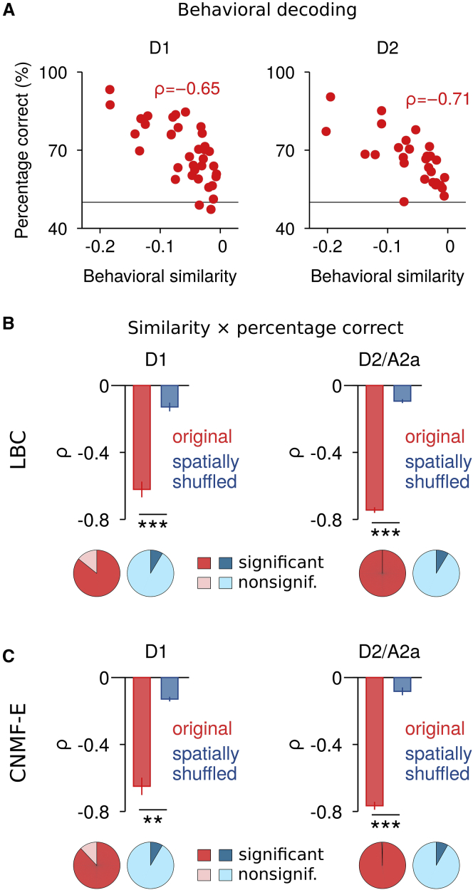
Figureu00a05
Behavior Decoding Based on SPN Ensemble Activity (A) Relationship between behavioral similarity and decoding performance of a support vector machine (SVM) for binary classification. The decoding perfo...
Figure images are served from the NIH/NLM PubMed Central Open Access Subset or Europe PMC; copyright remains with the publishers and authors.
💬 Discussion
0 commentsNo comments yet. Be the first to start a discussion!
Leave a Comment