Abstract
AbstractDNA is a compelling alternative to non-volatile information storage technologies due to its information density, stability, and energy efficiency. Previous studies have used artificially synthesized DNA to store data and automated next-generation sequencing to read it back. Here, we report digital Nucleic Acid Memory (dNAM) for applications that require a limited amount of data to have high information density, redundancy, and copy number. In dNAM, data is encoded by selecting combinations of single-stranded DNA with (1) or without (0) docking-site domains. When self-assembled with scaffold DNA, staple strands form DNA origami breadboards. Information encoded into the breadboards is read by monitoring the binding of fluorescent imager probes using DNA-PAINT super-resolution microscopy. To enhance data retention, a multi-layer error correction scheme that combines fountain and bi-level parity codes is used. As a prototype, fifteen origami encoded with ‘Data is in our DNA!n’ are analyzed. Each origami encodes unique data-droplet, index, orientation, and error-correction information. The error-correction algorithms fully recover the message when individual docking sites, or entire origami, are missing. Unlike other approaches to DNA-based data storage, reading dNAM does not require sequencing. As such, it offers an additional path to explore the advantages and disadvantages of DNA as an emerging memory material.
🔬 Techniques
💻 Software
✨ Fluorophores
🧪 Sample Preparation
🏭 Microscope Brands
🧪 Reagent Suppliers
📷 Detectors
💻 Software Details
🏛️ Research Organizations (ROR)
Affiliated research institutions:
📋 Methods
The materials purchased for this study, and their respective vendors, are outlined in Table 1 . All other reagents were obtained from Sigma. Table 1 Materials. Materials purchased Vendor DNA staple strands Integrated DNA Technologies M13 bacteriophage single-stranded DNA scaffolds (M13mp18) Bayou Biolabs Cy3B-labeled DNA oligonucleotide (M1 Imager strand: CTAGATGTAT-Cy3B) Bio-Synthesis, Inc. 150 nm diameter silanized gold nanoparticles (AuNPs) Nanopartz Glass coverslips Ted Pella, Inc. Sticky-slide flow cells (sticky-Slide I 0.2 Luer) Ibidi Liquinox Pollardwater, Inc. MilliporeSigma MilliporeSigma Protocatechuate 3,4-dioxygenase pseudomonas (PCD) MilliporeSigma (+−)−6-hydroxy-2,5,7,8-tetra-methylchromane-2-carboxylic acid (Trolox) MilliporeSigma MgCl 2 MilliporeSigma Nuclease-free water Thermo Fisher Scientific Tris-borate-EDTA (TBE) Thermo Fisher Scientific Tris-Acetate-EDTA (TAE) Thermo Fisher Scientific List of materials and vendors used in this study. Buffers As previously described 17 , two buffers were used to prepare and image DNA origami: a deposition buffer and an imaging buffer. The deposition buffer contained 0.5× TBE and 18 mM MgCl 2 . The imaging buffer contained the deposition buffer with the supplement of 60 nM PCD, 1 mM Trolox, 3 nM imager strands, and 10 mM PCA. PCA was added to the imaging buffer immediately before the start of a DNA-PAINT recording.
Encoding algorithm
The encoding algorithm used a multi-layer error correction scheme to encode message data bits along with the index, orientation, and error correction bits onto multiple origami (Fig. S4 ). At the message level, the algorithm used a fountain code to encode the data. Let m be a message string composed of a sequence of n bits. The fountain code algorithm first divides m into k equally sized and non-overlapping substrings s 1 , s 2 , …, s k , where the concatenation s 1 s 2 … s k = m , and then systematically combines one to many segments using the binary XOR operation to form multiple data blocks called droplets. The number of segments d used to form each droplet are typically drawn from a distribution based on the Soliton distribution: 1 documentclass[12pt]{minimal} usepackage{amsmath} usepackage{wasysym} usepackage{amsfonts} usepackage{amssymb} usepackage{amsbsy} usepackage{mathrsfs} usepackage{upgreek} setlength{oddsidemargin}{-69pt} begin{document}$$pleft( 1 right) = 1/k$$end{document} p 1 = 1 / k The Soliton distribution ensures that the algorithm encodes the optimal number of single-segment droplets necessary for the decode step. Once the number of segments d for a droplet is determined, the droplet is formed by XOR’ing d randomly selected, unique segments from m , with each segment being selected with probability 1/ k . For our experiments, we divided the message ‘Data is in our DNA!n’ into 10 segments of 16 bits each. The segments were then combined via an XOR in different combinations using the fountain code algorithm to form the 15 droplets. While the theoretical minimum number of 16-bit droplets required to decode the message is 10, the redundancy provided by the additional droplets ensured that the message would be recoverable in all cases involving the loss of one droplet, and in some cases with the loss of up to five droplets (Fig. 4 ). After generating the droplets using fountain codes, the encoding algorithm encoded each droplet onto fifteen 6 × 8 matrixes, and sequentially added index and orientation marker bits, computed and added checksum bits, and then added parity bits (Fig. 1b ). These matrixes were used to construct 15 origami structures, with a one-to-one mapping between the matrixes and the origami’s data domains. Figure 1b shows the layout of how droplet information was encoded onto each origami, composed of 16 bits of droplet data (green coloring in Fig. 1b ), four indexing bits (red), four orientation bits (magenta), four checksum bits (yellow), and twenty parity bits (blue). It is important to note that the layout of the data, orientation, and index bits relative to the corresponding parity and checksum bits is invariant to rotation, which made it possible for the error correction algorithm to perform error detection and recovery before determining the orientation (Fig. S4 ). This led to more robust data recovery.
Show full methods section
The materials purchased for this study, and their respective vendors, are outlined in Table 1 . All other reagents were obtained from Sigma. Table 1 Materials. Materials purchased Vendor DNA staple strands Integrated DNA Technologies M13 bacteriophage single-stranded DNA scaffolds (M13mp18) Bayou Biolabs Cy3B-labeled DNA oligonucleotide (M1 Imager strand: CTAGATGTAT-Cy3B) Bio-Synthesis, Inc. 150 nm diameter silanized gold nanoparticles (AuNPs) Nanopartz Glass coverslips Ted Pella, Inc. Sticky-slide flow cells (sticky-Slide I 0.2 Luer) Ibidi Liquinox Pollardwater, Inc. MilliporeSigma MilliporeSigma Protocatechuate 3,4-dioxygenase pseudomonas (PCD) MilliporeSigma (+−)−6-hydroxy-2,5,7,8-tetra-methylchromane-2-carboxylic acid (Trolox) MilliporeSigma MgCl 2 MilliporeSigma Nuclease-free water Thermo Fisher Scientific Tris-borate-EDTA (TBE) Thermo Fisher Scientific Tris-Acetate-EDTA (TAE) Thermo Fisher Scientific List of materials and vendors used in this study. Buffers As previously described 17 , two buffers were used to prepare and image DNA origami: a deposition buffer and an imaging buffer. The deposition buffer contained 0.5× TBE and 18 mM MgCl 2 . The imaging buffer contained the deposition buffer with the supplement of 60 nM PCD, 1 mM Trolox, 3 nM imager strands, and 10 mM PCA. PCA was added to the imaging buffer immediately before the start of a DNA-PAINT recording.
Encoding algorithm
The encoding algorithm used a multi-layer error correction scheme to encode message data bits along with the index, orientation, and error correction bits onto multiple origami (Fig. S4 ). At the message level, the algorithm used a fountain code to encode the data. Let m be a message string composed of a sequence of n bits. The fountain code algorithm first divides m into k equally sized and non-overlapping substrings s 1 , s 2 , …, s k , where the concatenation s 1 s 2 … s k = m , and then systematically combines one to many segments using the binary XOR operation to form multiple data blocks called droplets. The number of segments d used to form each droplet are typically drawn from a distribution based on the Soliton distribution: 1 documentclass[12pt]{minimal} usepackage{amsmath} usepackage{wasysym} usepackage{amsfonts} usepackage{amssymb} usepackage{amsbsy} usepackage{mathrsfs} usepackage{upgreek} setlength{oddsidemargin}{-69pt} begin{document}$$pleft( 1 right) = 1/k$$end{document} p 1 = 1 / k The Soliton distribution ensures that the algorithm encodes the optimal number of single-segment droplets necessary for the decode step. Once the number of segments d for a droplet is determined, the droplet is formed by XOR’ing d randomly selected, unique segments from m , with each segment being selected with probability 1/ k . For our experiments, we divided the message ‘Data is in our DNA!n’ into 10 segments of 16 bits each. The segments were then combined via an XOR in different combinations using the fountain code algorithm to form the 15 droplets. While the theoretical minimum number of 16-bit droplets required to decode the message is 10, the redundancy provided by the additional droplets ensured that the message would be recoverable in all cases involving the loss of one droplet, and in some cases with the loss of up to five droplets (Fig. 4 ). After generating the droplets using fountain codes, the encoding algorithm encoded each droplet onto fifteen 6 × 8 matrixes, and sequentially added index and orientation marker bits, computed and added checksum bits, and then added parity bits (Fig. 1b ). These matrixes were used to construct 15 origami structures, with a one-to-one mapping between the matrixes and the origami’s data domains. Figure 1b shows the layout of how droplet information was encoded onto each origami, composed of 16 bits of droplet data (green coloring in Fig. 1b ), four indexing bits (red), four orientation bits (magenta), four checksum bits (yellow), and twenty parity bits (blue). It is important to note that the layout of the data, orientation, and index bits relative to the corresponding parity and checksum bits is invariant to rotation, which made it possible for the error correction algorithm to perform error detection and recovery before determining the orientation (Fig. S4 ). This led to more robust data recovery.
DNA origami folding Rectangular
DNA origami structures (~90 × 70 nm) were designed based on previous work by Rafat et al. 30 with 48 potential docking strand sites arranged in a 6 × 8 matrix with 10 nm spacing. Then, using the protocol described by Schnitzbauer et al. 17 a mixture of extended and unmodified staple strands (SI Tables S1 and S2 ) were selected to fold the M13 scaffold into the designed shape, with extended strands located at the ‘1’ positions described in the design matrix (SI Table S4 ). As described in the introduction, an extended staple strand has a binding site for the M1 imager strand, unmodified strands bind solely to the scaffold DNA to induce folding. Using this method, 15 origami designs were created that matched the 15 matrixes output by the encoding algorithm. We assembled individual origami designs by combining 22 nM M13mp18 with 10× unmodified stands, 50× extended strands, 1× TAE and 18 mM MgCl 2 (in nuclease-free water; 100 µL total volume) and folding in a Mastercycler nexus thermal cycler (Eppendorf) using the following heating cycle: [1 min 90 °C, 2 min 80 °C, then from 80 °C to 25 °C over 12 h]. We purified the origami by running them on an ice-cooled 0.8% agarose gel containing 0.5× TBE and 8 mM MgCl 2 , excising the single sharp band, and collecting the exudate of the crushed gel piece. Sharp triangle origami used as fiducial markers were prepared similarly, as previously described 31 (see S1 Table S3 for oligonucleotide sequences). All purified origami were stored in the dark at 4 °C until use.
Glass coverslip preparation
Borosilicate glass coverslips (25 × 75 and 22 × 22 mm, #1 Gold Seal Coverglass) were sonicated in 0.1% (v/v) Liquinox and nano-pure water (1 min in each) to remove contaminants and dried at 40 °C for at least 30 min. Fiducial markers (200 µL of 0.2 pM AuNPs) were deposited onto the coverslips for 10 min at room temperature. The labeled coverslips were rinsed with methanol and nano-pure water and stored at 40 °C prior to use.
DNA origami deposition onto coverslips
The glow discharge technique previously described by Green 24 was used to deposit DNA origami onto glass coverslips using an air-plasma vacuum glow-discharge system. Briefly, coverslips that had been cleaned and labeled with fiducial markers were exposed to glow discharge generated using an electrode coupled 115 V Electro-Technic BD-10A High-Frequency Generator under 2 Torr of vacuum for 75 s. For DNA-PAINT analysis, a sticky-Slide flow cell (~50 µL channel volume) was glued to the coverslip, DNA origami were then deposited by introducing 200 µL of 0.05 nM origami (a mixture of dNAM origami and sharp triangle origami 31 added as additional fiducial markers, in deposition buffer) into the flow chamber and incubated for 30 min at room temperature. After deposition, the flow chamber was rinsed with 1 mL of deposition buffer (no DNA origami) and refilled with imaging buffer. When performing AFM measurements on samples previously used for DNA-PAINT, a custom fluid chamber, modified from Jungmann et al. 32 , was used. A 22 × 22 mm coverslip was glued to a microscope slide using double-sided sticky tape with the addition of a thin layer of gel sealant—to both seal any gaps and weaken the binding of tape to the glass. Once DNA-PAINT imaging had been performed the sealant allowed the coverslip to be easily removed for further AFM analysis.
Fluorescence microscopy
DNA origami was imaged below the diffraction limit of light via DNA-PAINT 17 using an inverted Nikon Eclipse Ti2 microscope from Nikon Instruments in total internal reflectance fluorescence (TIRF) mode. The images were acquired using: an optical feedback focal-drift correction system developed in-house or the Perfect Focus System from Nikon Instruments; an oil-immersion CFI Apochromat ×100 TIRF objective with a 1.49 numerical aperture, plus an extra ×1.5 magnification from Nikon Instruments; and a 405/488/561/647 nm Laser Quad Band Set TIRF filter cube from Chroma. A 561 nm laser source excited fluorescence from the DNA-PAINT imager strands within an evanescent field extending a few hundred nanometers above the surface of the glass coverslip. The emitted fluorescence was imaged onto the full chip with 512 × 512 pixels (1 pixel = 16 μm) using a ProEM EMCCD camera from Princeton Instruments at a 300 ms exposure time (~3 frames/s). During an experimental recording, each of the individual data strands, within a dNAM origami’s matrix, transiently and repeatedly bound an imager strand, which emits a signal, creating a series of blinks. Images with blinking events were recorded into a stack (typically 40,000 frames per recording) using Nikon NIS-Elements version 5.20.00 (Nikon Instruments) or LightField version 5 (Princeton Instruments) prior to processing and analysis.
DNA-PAINT fluorophore localization
After recording a DNA-PAINT stack, the center position of signals (localizations) emitted by imager probes, transiently binding to DNA origami docking strands, were identified using the ImageJ ThunderSTORM plugin 33 . The localizations were rendered and then drift corrected using the Picasso-Render software package, as described by Schnitzbauer et al. 17 . Data visualization and peak fitting of image data for PSF analysis were performed using OriginPro Version 2019b (OriginLab).
Localization data processing
A custom algorithm was developed for identifying clusters of localizations, determining the maximum likelihood position of the emitters, and generating binary matrix data. The algorithm selected localization clusters at random from the localization list. To do this, it sampled random points in the list, determined the average position of nearby localizations, and counted the localizations within a radius ( R ) and the localizations within a band R < r < 2 R . The algorithm accepted clusters if the counts in the inner circle were greater than a threshold and the counts in the outer band were less than 15% of the counts in the inner band. This ensured selection of bright clusters that were isolated from other clusters. The algorithm then fits the cluster localizations to a grid of emitters. An idealized grid was created using the average DNA-PAINT image produced by several thousand individual origami structures of the same architecture used in this work. The algorithm performed fitting using a maximum likelihood estimation for the likelihood function: 2 documentclass[12pt]{minimal} usepackage{amsmath} usepackage{wasysym} usepackage{amsfonts} usepackage{amssymb} usepackage{amsbsy} usepackage{mathrsfs} usepackage{upgreek} setlength{oddsidemargin}{-69pt} begin{document}$$Lleft( {I,x_c,y_c,theta ,{mathrm{{Delta}}}x_g^2,B} right) = mathop {prod }limits_i left( {mathop {sum }limits_k frac{{I_k}}{a}exp left( { - frac{{left( {x_i - x_kleft( {x_c,y_c,theta } right)} right)^2 + left( {y_i - y_kleft( {x_c,y_c,theta } right)} right)^2}}{{{mathrm{{Delta}}}x_i^2 + {mathrm{{Delta}}}x_g^2}}} right)} right) ast frac{B}{A} ast P(N,I,B)$$end{document} L I , x c , y c , θ , Δ x g 2 , B = ∏ i ∑ k I k a exp − x i − x k x c , y c , θ 2 + y i − y k x c , y c , θ 2 Δ x i 2 + Δ x g 2 * B A * P ( N , I , B ) Where I k is the intensity of the k th emitter, ( x c , y c ) is the center position of the grid, θ is the rotation angle of the grid, Δ x g is the global lateral uncertainty caused by an error in drift correction, B is the background, Δ x i is the lateral position uncertainty of localization i reported by the ThunderSTORM analysis described above, ( x i , y i ) is the position of the i th localization, ( x k , y k ) is the position of the k th emitter, as a function of the center position and rotation of the grid, A is the area of the cluster, and N is the number of localizations found in the cluster. a is a normalization constant given by: 3 documentclass[12pt]{minimal} usepackage{amsmath} usepackage{wasysym} usepackage{amsfonts} usepackage{amssymb} usepackage{amsbsy} usepackage{mathrsfs} usepackage{upgreek} setlength{oddsidemargin}{-69pt} begin{document}$$a = 2pi left( {{mathrm{{Delta}}}x_i^2 + {mathrm{{Delta}}}x_g^2} right)$$end{document} a = 2 π Δ x i 2 + Δ x g 2 P(N,I,B) is the probability of finding N localizations given the intensity of each grid point and the background intensity, determined from the Poisson distribution of mean value N . This likelihood function determines the probability of finding localizations at all of the observed sites given a set of point emitters at the grid sites with intensity I k and background intensity B . The optimization utilized the L-BFGS-B method of the minimize function provided by Scipy 34 to minimize −log (L) subject to the constraint that all intensities are positive. Signals that did not align to the 6 × 8 grid were filtered to minimize fragmented origami and to reduce inadvertent assimilation of the triangular origami fiducial markers into the results. The algorithm then assigned the emitters a binary value (1 or 0) using an empirically derived threshold value. This binary matrix data was decoded using the decoding algorithm described below. In parallel with this blind cluster analysis, the processing algorithm also carried out a template matching step to more reliably identify individual origami and analyze their errors. This additional step used the known origami designs as templates, matching the observed origami to the best fit, based on the total number of errors. This method was more robust to higher error rates than the blind cluster analysis and allowed more origami to be identified for image averaging and error analysis (Fig. 3 ). It should be noted, however, that the template matching method cannot be considered as a data reading method because it requires a priori knowledge of the data being analyzed. For this reason, none of the analysis of the recovery rates or data density discussed here used data obtained from pattern matching.
Decoding algorithm
The decoding algorithm (Fig. S5 ) utilized a multi-layer error correction/encoding scheme to recover the data in the presence of errors. The algorithm first works at the dNAM origami level (Step 1, below), using the parity and checksum bits, to attempt to identify and correct errors and recover the correct matrix. After recovery, the algorithm uses binary operations to recover the original data segments from the droplets (Step 2, below). Decoding algorithm: Step 1–error correction Given raw binary matrix data M for a single dNAM origami, the output from the localization data processing step, the matrix decoding algorithm determined which, if any, bits were associated with checksum and parity errors by calculating the bi-level matrix parity and checksum values, as described in Fig. S4 . Any discrepancies between the calculated parity and checksum values and the values recovered from the origami were noted, and a weight for each of the bits associated with the errant parity/checksum calculation was deduced. If no parity/checksum errors were detected for a particular matrix, then the data was assumed to be accurate, and the algorithm proceeded to extract the message data. To determine the site(s) of likely errors, the decoding algorithm first determined a weight for every cell in M , beginning with data cells (the cells containing droplet, index, or orientation bits) and proceeding to parity and checksum cells. Let documentclass[12pt]{minimal} usepackage{amsmath} usepackage{wasysym} usepackage{amsfonts} usepackage{amssymb} usepackage{amsbsy} usepackage{mathrsfs} usepackage{upgreek} setlength{oddsidemargin}{-69pt} begin{document}$$P_{c_{ij}}$$end{document} P c i j be the set of parity functions calculated over a given data cell c ij . Then for each data cell c ij : 4 documentclass[12pt]{minimal} usepackage{amsmath} usepackage{wasysym} usepackage{amsfonts} usepackage{amssymb} usepackage{amsbsy} usepackage{mathrsfs} usepackage{upgreek} setlength{oddsidemargin}{-69pt} begin{document}$$x_{ij} = mathop {sum }limits_{f_{c_{pq}} in P_{c_{ij}}} left| {c_{pq} - f_{c_{pq}}left( {mathbf{M}} right)} right|$$end{document} x i j = ∑ f c p q ∈ P c i j c p q − f c p q M Where c pq is the parity cell where the expected binary value of f is stored. The weight for each parity cell c ij was then calculated based on the number of non-zero weights greater than 1 for the data cells associated with it. More formally, let c ij be a parity cell and documentclass[12pt]{minimal} usepackage{amsmath} usepackage{wasysym} usepackage{amsfonts} usepackage{amssymb} usepackage{amsbsy} usepackage{mathrsfs} usepackage{upgreek} setlength{oddsidemargin}{-69pt} begin{document}$$D_{c_{ij}}$$end{document} D c i j be the set of data cells used in the calculation of c ij . Then the weight x ij for each parity cell c ij is: 5 documentclass[12pt]{minimal} usepackage{amsmath} usepackage{wasysym} usepackage{amsfonts} usepackage{amssymb} usepackage{amsbsy} usepackage{mathrsfs} usepackage{upgreek} setlength{oddsidemargin}{-69pt} begin{document}$$x_{ij} = mathop {sum }limits_{c_{pq} in D_{c_{ij} wedge x_{pq} > 1}} {mathop{rm{sgn}}} left( {x_{pq}} right)$$end{document} x i j = ∑ c p q ∈ D c i j ∧ x p q > 1 sgn x p q The higher the weight value, the higher the probability that the corresponding cell had an error. An overall score for the matrix was then calculated by summing over all x ij and normalizing by the sum of the correctly matched parity bits. This value was designated as the overall weight of the matrix. Higher values of this weight correspond to matrixes with more errors. 6 documentclass[12pt]{minimal} usepackage{amsmath} usepackage{wasysym} usepackage{amsfonts} usepackage{amssymb} usepackage{amsbsy} usepackage{mathrsfs} usepackage{upgreek} setlength{oddsidemargin}{-69pt} begin{document}$${mathrm{Overall}},{mathrm{matrix}},{mathrm{weight}} = frac{{mathop {sum }nolimits_{i = 0}^6 mathop {sum }nolimits_{j = 0}^8 x_{ij}}}{{# {mathrm{number}},{mathrm{of}},{mathrm{matched}},{mathrm{parity}},{mathrm{bits}}}}$$end{document} Overall matrix weight = ∑ i = 0 6 ∑ j = 0 8 x i j # number of matched parity bits The algorithm then performed a greedy search to correct the errors using a priority queue ordered by the overall matrix weight (Fig. S6 ). The algorithm began by iteratively altering each of the probable site errors and computing the overall matrix weight of the modified matrix for each, placing each potential bit flip into a priority queue where the flips that produced the lowest overall weights had the highest priority. At each step, the algorithm selected the bit flip associated with the highest priority in the queue and then repeated this process on the resulting matrix. This process was continued until the algorithm produced a matrix with no mismatches or until it reached the maximum number of allowed bit flips (9 for our simulation/experiment). If it reached the maximum number of flips, it returned to the queue to pursue the next highest priority path. If the algorithm found a matrix with no mismatches, it then checked the orientation bits and oriented the matrix accordingly. The droplet and index data were then extracted and passed to the next step. If the queue was emptied without finding a correct matrix, the algorithm terminated in failure. Decoding algorithm: Step 2–fountain code decoding After extracting the droplet and index data from multiple origami the algorithm attempted to recover the full message (Fig. S7 ). Once decoded, each droplet had one or multiple segments XORed in it. Using the recovered indexes the algorithm determined how many and which segments were contained in each droplet. To decode the message, the algorithm maintained a priority queue of droplets based on the number of segments they contained (their degree), with the lowest degree droplets having the highest priority. The algorithm looped through the queue, removing the lowest degree droplet, attempting to use it to reduce the degree of the remaining droplets using XOR operations, and re-queuing the resulting droplets. Upon finding a droplet of ‘degree one’ it stored it as a segment for the final message. If all segments were recovered, the algorithm terminated successfully.
Data simulation test
To test the robustness of our encoding and decoding algorithms, origami data were simulated with randomly generated messages and errors. First, random binary messages of size m were created (for m = 160 to 12,800 bits, at 320-bit intervals). These messages were then divided into m/b equally sized segments, where b is the number of data bits to be encoded onto an individual origami. For fixed-size origami, larger messages necessitated a smaller b , as more bits had to be dedicated to the index. In these cases, b varied between eight (for m = 12,800) and twelve (for m = 160). After determining message segments, droplets were formed using the fountain code algorithm and encoded onto origami, along with the corresponding index, orientation, and error-correcting bits. Ten in silico copies of each unique origami were created, and 0–9 bits flipped at random to introduce errors. The origami was decoded as described above. Reporting summary Further information on research design is available in the Nature Research Reporting Summary linked to this article.
Supplementary information Supplementary Information Peer Review File Reporting Summary
📊 Figures
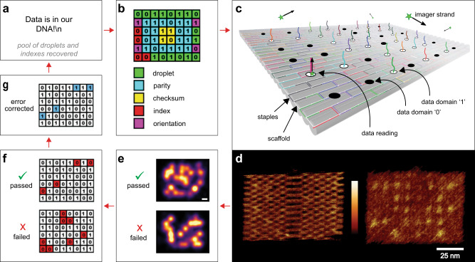
Fig. 1
Binary dNAM overview.
The test message ( a ) for optically reading dNAM was u2018Data is in our DNA!u2019. The message was encoded and then synthesized into 15 dNAM origami. For clarity, only one of the 15 designs is shown...
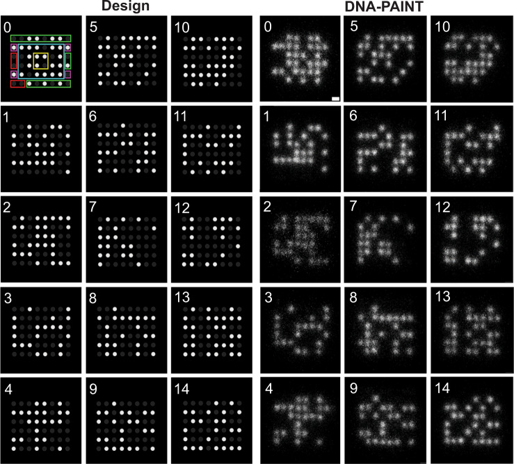
Fig. 2
DNA-PAINT imaging of dNAM indicates all sites are recovered in a single read.
dNAM origami from a DNA-PAINT recording were identified and classified by aligning and template matching them with the 15 design matrixes (Design) in which all potential docking sites are shown. Fille...
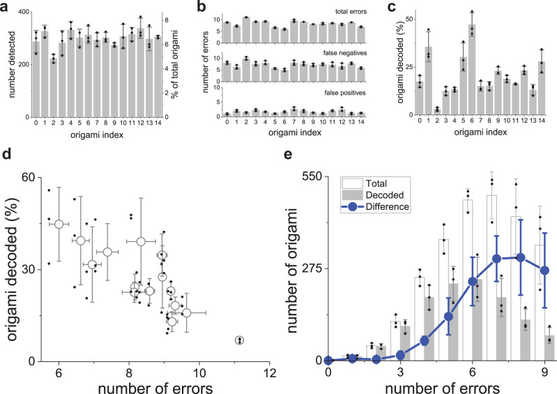
Fig. 3
All 15 dNAM data strings were recovered from a single read.
(a) plots the numbers of each origami index observed in a single recording, based on template matching. The mean counts are shown as gray bars, with the percentage of the total origami indicated on th...
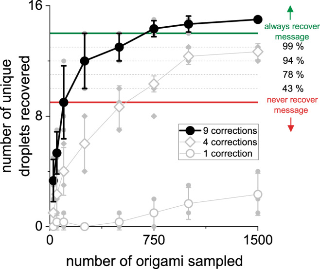
Fig. 4
Number of dNAM origami required to recover the message.
The mean number of unique dNAM origami correctly decoded for randomly selected subsamples of decoded binary stringsu00a0are shown. The analysis was broken out by the number of errors corrected for eac...
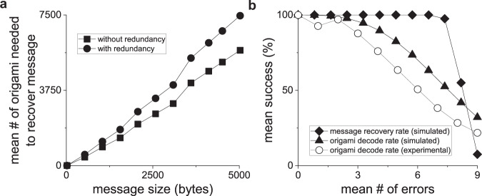
Fig. 5
dNAM origami and message recovery rates in the presence of increasing errors.
Simulations were performed to determine the theoretical success rates for correctly decoding individual dNAM origami and recovering encoded messages. In ( a ), the mean number of dNAM origami needed t...
Figure images are served from the NIH/NLM PubMed Central Open Access Subset or Europe PMC; copyright remains with the publishers and authors.
💬 Discussion
0 commentsNo comments yet. Be the first to start a discussion!
Leave a Comment