Abstract
Basal forebrain cholinergic neurons (BFCNs) project throughout the cortex to regulate arousal, stimulus salience, plasticity, and learning. Although often treated as a monolithic structure, the basal forebrain features distinct connectivity along its rostrocaudal axis that could impart regional differences in BFCN processing. Here, we performed simultaneous bulk calcium imaging from rostral and caudal BFCNs over a 1-month period of variable reinforcement learning in mice. BFCNs in both regions showed equivalently weak responses to unconditioned visual stimuli and anticipated rewards. Rostral BFCNs in the horizontal limb of the diagonal band were more responsive to reward omission, more accurately classified behavioral outcomes, and more closely tracked fluctuations in pupil-indexed global brain state. Caudal tail BFCNs in globus pallidus and substantia innominata were more responsive to unconditioned auditory stimuli, orofacial movements, aversive reinforcement, and showed robust associative plasticity for punishment-predicting cues. These results identify a functional topography that diversifies cholinergic modulatory signals broadcast to downstream brain regions.
🔬 Techniques
🧬 Organisms
✨ Fluorophores
🧪 Sample Preparation
🏭 Microscope Brands
🧪 Reagent Suppliers
💻 Software Details
💾 Data Repositories
🏷️ Research Resource Identifiers (RRIDs)
Verified research resources used in this paper:
🏛️ Research Organizations (ROR)
Affiliated research institutions:
📋 Methods
Key resources table
Reagent type (species) or resource Designation Source or reference Identifiers Additional information Genetic reagent ( Mus musculus ) B6.129S- Chat tm1(cre)Lowl /MwarJ Jackson Laboratory RRID: IMSR_JAX:031661 Male Genetic reagent ( Mus musculus ) B6.Cg-Igs7 tm148.1(tetO-GCaMP6f,CAG-tTA2)Hze /J Jackson Laboratory RRID: IMSR_JAX:030328 Female Antibody Anti-ChAT (goat polyclonal) Millipore Sigma Cat #: AB144PRRID: AB_2079751 (1:100) Antibody Anti-Goat (donkey polyclonal) Abcam Cat#: AB150132RRID: AB_2810222 (1:500) Recombinant DNA reagent ACh sensor Dr Yulong Li GRAB ACh 3.0 Software, algorithm Labview National Instruments RRID: SCR_014325 Version 2015 Software, algorithm MATLAB Mathworks RRID: SCR_001622 Version R2021a Other DAPI stain Vectorlabs Cat #: H-1500–10RRID: AB_2336788 Other Allen Brain Atlas Lein et al., 2007 RRID: SCR_013286 Animals All procedures were approved by the Massachusetts Eye and Ear Animal Care and Use Committee and followed the guidelines established by the National Institutes of Health for the care and use of laboratory animals. Male ChAT-cre-∆Neo (homozygous, Jackson Labs 031661) and female Ai148 mice (hemizygous, Jackson Labs 030328) were bred in-house to generate mice of both sexes for this study. Offspring were therefore hemizygous for ChAT-cre-∆Neo and either had hemizygous expression of cre-dependent GCaMP6f (ChAT+/GCaMP+) or did not express GCaMP (ChAT+/GCaMP-). Offspring genotypes were confirmed by PCR (Transnetyx probes) and by histology following perfusion. Experiments were performed in adult mice, 2–3 months of age at the time the first measurement was performed. Prior to behavioral testing, mice were maintained on a 12 hr light/12 hr dark cycle with ad libitum access to food and water. Mice were grouped-housed unless they had undergone a major survival surgery. Dual fiber imaging of ChAT neuron GCaMP fluorescence in GP/SI and HDB was performed in 11 ChAT+/GCaMP+ mice, four of which were used for additional histological quantification. Fiber imaging of ACh3.0 sensor fluorescence in ACtx was performed in 10 ChAT+/GCaMP- mice.
Show full methods section
Key resources table
Reagent type (species) or resource Designation Source or reference Identifiers Additional information Genetic reagent ( Mus musculus ) B6.129S- Chat tm1(cre)Lowl /MwarJ Jackson Laboratory RRID: IMSR_JAX:031661 Male Genetic reagent ( Mus musculus ) B6.Cg-Igs7 tm148.1(tetO-GCaMP6f,CAG-tTA2)Hze /J Jackson Laboratory RRID: IMSR_JAX:030328 Female Antibody Anti-ChAT (goat polyclonal) Millipore Sigma Cat #: AB144PRRID: AB_2079751 (1:100) Antibody Anti-Goat (donkey polyclonal) Abcam Cat#: AB150132RRID: AB_2810222 (1:500) Recombinant DNA reagent ACh sensor Dr Yulong Li GRAB ACh 3.0 Software, algorithm Labview National Instruments RRID: SCR_014325 Version 2015 Software, algorithm MATLAB Mathworks RRID: SCR_001622 Version R2021a Other DAPI stain Vectorlabs Cat #: H-1500–10RRID: AB_2336788 Other Allen Brain Atlas Lein et al., 2007 RRID: SCR_013286 Animals All procedures were approved by the Massachusetts Eye and Ear Animal Care and Use Committee and followed the guidelines established by the National Institutes of Health for the care and use of laboratory animals. Male ChAT-cre-∆Neo (homozygous, Jackson Labs 031661) and female Ai148 mice (hemizygous, Jackson Labs 030328) were bred in-house to generate mice of both sexes for this study. Offspring were therefore hemizygous for ChAT-cre-∆Neo and either had hemizygous expression of cre-dependent GCaMP6f (ChAT+/GCaMP+) or did not express GCaMP (ChAT+/GCaMP-). Offspring genotypes were confirmed by PCR (Transnetyx probes) and by histology following perfusion. Experiments were performed in adult mice, 2–3 months of age at the time the first measurement was performed. Prior to behavioral testing, mice were maintained on a 12 hr light/12 hr dark cycle with ad libitum access to food and water. Mice were grouped-housed unless they had undergone a major survival surgery. Dual fiber imaging of ChAT neuron GCaMP fluorescence in GP/SI and HDB was performed in 11 ChAT+/GCaMP+ mice, four of which were used for additional histological quantification. Fiber imaging of ACh3.0 sensor fluorescence in ACtx was performed in 10 ChAT+/GCaMP- mice.
Surgical procedure for GCaMP photometry
Mice were anesthetized with isoflurane in oxygen (5% induction, 2% maintenance) and placed in a stereotaxic frame (Kopf Model 1900). A homeothermic blanket system was used to maintain body temperature at 36.6° (FHC). Lidocaine hydrochloride was administered subcutaneously to numb the scalp. The dorsal surface of the scalp was retracted and the periosteum was removed. Dual optic fiber implants (Doric, 400 μm core, NA 0.48, 1.25 mm diameter low-autofluorescence metal ferrule) were slowly lowered into HDB (0.9 × 0.3 × 4.7) and GP/SI (2.5 × –1.5 × 3.3 mm from bregma, [lateral × caudal × ventral]) in the right hemisphere. Silicon adhesive (WPI Kwik-Sil) was applied to the exposed brain surface. The exposed skull surface was prepped with etchant (C&B metabond) and 70% ethanol before affixing a titanium head plate (iMaterialise) to the skull with dental cement (C&B Metabond). At the conclusion of the procedure, Buprenex (0.05 mg/kg) and meloxicam (0.1 mg/kg) were administered and the animal was transferred to a warmed recovery chamber.
Surgical procedure for ACh sensor photometry
The initial surgical procedures and perioperative care were similar to that for GCaMP photometry. The skull overlying the right ACtx exposed by moving the temporalis muscle. A burr hole was made on the temporal ridge at 2.9 mm posterior to bregma, using a 31-gauge needle. A motorized injection system (Stoelting) was used to inject 200 nL of AAV9-hSyn-ACh3.0 (diluted 10% in sterile saline from 3.45 × 10 13 genome copies/mL) via a pulled glass micropipette 0.5 mm below the pial surface. We waited at least 10 min following the injection before withdrawing the micropipette. A tapered fiber (Optogenix, NA 0.39, diameter 200 µm, active length 1.0 mm) was implanted 1 mm below the pial surface and secured using dental cement dyed with India Ink, which also secured the titanium head plate. Sensor photometry experiments began 3 weeks following the injection. Pupillometry Mice were placed in an electrically conductive cradle and habituated to head fixation during three sessions of 15, 30, and 60 min over 3 consecutive days. Video recordings of the pupil under isoluminous background conditions were performed during the final habituation session and the following sensory characterization day. Video recordings were made at 30 Hz with a CMOS camera (Teledyne Dalsa, model M2020) outfitted with a lens (Tamron 032938) and infrared longpass filter (Midopt lp830-25.5). Automated analysis of pupil diameter follows the procedure described previously by McGinley et al., 2015a . Briefly, each movie was thresholded such that most pixel values within the pupil were below threshold and all other pixels were above threshold. A circle was fit to the pupil by first calculating the center of mass within the pupil and then centering a circle with the corresponding area to that point. Canny edge detection was then used to identify edge pixels within each grayscale image. Edge pixels were removed if they were more than three pixels away from a pupil pixel or outside of an annulus with diameters that were 0.5 and 1.75 the diameter of the initial fit circle. As a final step, an ellipse was fit to the remaining edge pixels using least-squares regression and the pupil diameter was defined from the diameter of a circle with a matching area. This procedure was performed for each image frame using a MATLAB (Mathworks) script adapted from the original publication ( McGinley et al., 2015a ). Pupil diameter for ACh3.0 sensor imaging experiments was extracted using DeepLabCut (version 2.1.8.2, Nath et al., 2019 ). Specifically, three investigators each labeled 100 frames taken from 10 mice, for a total of 300 frames from 30 mice. The four cardinal and four intercardinal compass points were marked for each pupil. Marker placement was confirmed by at least one additional investigator. Training was performed on 95% of frames. We used a ResNet-101 based neural network with default parameters for 1,030,000 training iterations. We then used a p-value cutoff of 0.9 to condition the X,Y coordinates for analysis. This network was then used to analyze videos from similar experimental settings from the 10 ACh3.0 sensor imaging mice. We calculated pupil diameter for each frame by fitting an ellipse to the identified pupil contour points using a least-squares criterion and calculating the long axis diameter.
Operant behavioral testing
All mice proceeded through the same series of tests beginning 2 weeks following fiber implant surgery ( Figure 2A ). On sessions 1 and 2, mice were habituated to head fixation and the body cradle. On session 3, pupillometry was performed without sensory stimulation. On session 4, pupillometry and fiber imaging was performed in response to the presentation of auditory or visual stimuli. Beginning on day 5, mice were placed on water restriction and were monitored until they reached 80% of their baseline weight. Beginning on day 8 or 9, after several days of behavioral shaping, mice began appetitive operant training that rewarded vigorous licking shortly following the presentation of three different tone frequencies. Finally, on days 13–22, mice were switched to a reinforcement reversal task, where two of the previously rewarded frequencies were switched to neutral or aversive reinforcement. These methods for each of these stages are provided in detail below.
Sensory characterization
Visual gratings were generated in MATLAB using the Psychtoolbox extension and presented via an 800 × 480 pixel display (Adafruit 2406) positioned approximately 15 cm from the left eye 45° off midline. Visual gratings were presented with a spatial frequency of 0.035 cycles per degree at three contrasts: 11%, 33%, and 100%. Gratings (2 s duration) were presented at both vertical and horizontal orientations. Spatial drift (2 Hz) was imposed along the orthogonal axis to orientation. Auditory stimuli were either pure tones or auditory drifting gratings (i.e., ripples). Stimuli were generated with a 24-bit digital-to-analog converter (National Instruments model PXI-4461) and presented via a free-field speaker (CUI, CMS0201KLX) placed approximately 10 cm from the left (contralateral) ear canal. Free-field stimuli were calibrated using a wide-band free-field microphone (PCB Electronics, 378C01). Pure tones were low (either 6 or 6.8 kHz), mid (9.5 or 11.3 kHz), or high (13.9 or 18.5 kHz) frequencies presented at three intensities (30, 50, and 70 dB SPL). Tones were 0.4 s duration shaped with 5 ms raised cosine onset and offset ramps. Auditory gratings ranged from 2 to 45 kHz with 2 s duration (5 ms raised cosine onset and offset ramps), presented at downward and upward frequency trajectories (at –2 and +2 Hz) at three intensities (30, 50, and 70 dB SPL). The spectrum was shaped with 20 frequency carriers per octave that were sinusoidally modulated with 90% depth at one cycle per octave. A single block consisted of 22 unique stimulus trials with a 7 s inter-trial interval (6 visual gratings [2 orientations × 3 contrasts], 9 tones [3 frequencies × 3 levels], 6 auditory gratings [2 directions × 3 intensities] and one silent trial where neither an auditory nor visual stimulus was presented). The stimulus order was randomly determined for each of 20 presentation blocks.
Operant training
Behavioral shaping for the rewarded tone detection task began after the sensory characterization session. In the initial phase of training, mice learned to vigorously lick a spout shortly following tone onset (low, mid, or high frequency, as specified above at 70 dB SPL) in order to receive a liquid reward (10% sucrose in water, 1.5 μL per reward, 1 reward per trial). Initially, tones were paired with rewards (i.e., Pavlovian conditioning), initiated 0.5 s after tone onset. Fiber imaging was not performed during behavioral shaping. Once mice were reliably licking prior to reward onset, the requirement to trigger reward delivery (i.e., operant conditioning) was progressively increased. The licking criterion to receive a reward was seven lickspout contacts within a 2.8 s period beginning 0.2 s after stimulus onset, where the interval between any 2 consecutive licks could not exceed 1 s. Individual trials were scored as hits, according to the criterion above, misses (no licks), or partial hits (lickspout contact that did not meet the criterion above). Intertrial intervals were determined randomly from a truncated exponential distribution within a range of 7–10 s. Trials were aborted in the event of lick spout contact in a withhold period of 2 s (initial phase) or 1.5 s (after reversal) preceding stimulus onset. Generally, mice learned to produce 7 licks in 2.8 s to initiate reward with low false alarm rates within two to three sessions. In order to analyze licking-related activity, separate lick bouts were also selected from the inter-trial periods. Lick bouts were defined as at least 2 lick contacts less than 250 ms apart, bookended by quiescent lick-free periods at least 1 s each before and after the bout. Once the reward rate exceeded 70% across all frequencies for at least one session, mice were transitioned to the reversal stage of the operant task in which one of the three tones remained associated with reward, one was associated with shock, and a third was not associated with reward or punishment (i.e., neutral outcome). The assignment of tone frequency to reinforcement condition was randomized across mice. Punishment was delivered by briefly electrifying the lick spout (0.6mA for 0.4 s) once the lick bout threshold (7 licks in 2.8 s) had been crossed. During this stage, the rewarded tone was presented on 50% of trials and the punished and neutral tones were each presented on 25% of trials. Operant testing was terminated once the Go probability stabilized across all tone frequencies for at least 2 consecutive days.
Fiber photometry Data acquisition
LEDs of different wavelengths provided a basis for separating calcium-dependent (465 nm) and calcium-independent (405 nm) fluorescence. Blue and purple LEDs were modulated at 210 and 330 Hz, respectively, and combined through an integrated fluorescence mini-cube (FMC4, Doric). The power at the tip of the patch cable was 0.1–0.2 mW. The optical patch cable was connected to the fiber implant via a zirconia mating sleeve. Bulk fluorescent signals were acquired with a femtowatt photoreceiver (2151, Newport) and digital signal processor (Tucker-Davis Technologies RZ5D). The signal was demodulated by the lock-in amplifier implemented in the processor, sampled at 1017 Hz, and low-pass filtered with a corner frequency at 20 Hz. The optical fibers were prebleached overnight by setting both LEDs to constant illumination at a low power (
📊 Figures
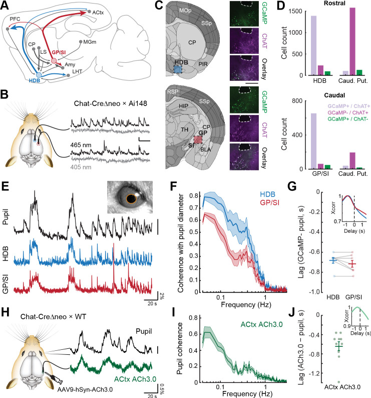
Figure 1.
Bulk basal forebrain cholinergic neuron (BFCN) activity and cortical acetylcholine release closely correspond with pupil-indexed global brain state.
( A ) Mid-sagittal diagram of the mouse brain depicting the diversity in major inputs (gray) and outputs (colored) between a rostroventral basal forebrain structure, the horizontal limb of the diagona...
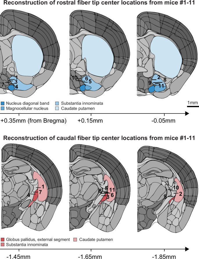
Figure 1u2014figure supplement 1.
Anatomical locations of horizontal limb of the diagonal band of Broca (HDB) and globus pallidus and substantia innominata (GP/SI) fiber tips.
The center of each 0.4 mm fiber implanted in rostral (top) and caudal (bottom) locations of the basal forebrain were identified in post-mortem sections of the 11 mice used throughout our study. Corona...
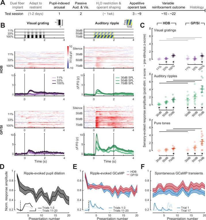
Figure 2.
Strong, rapidly habituating responses to unconditioned auditory - but not visual u2013 stimuli in globus pallidus and substantia innominata (GP/SI) cholinergic neurons.
( A ) Timeline for measurement sessions (black text) and procedures (gray text) performed in each of 11 ChAT-Cre-u0394neo u00d7 Ai148 mice. Basal forebrain cholinergic neuron (BFCN) responses to uncon...
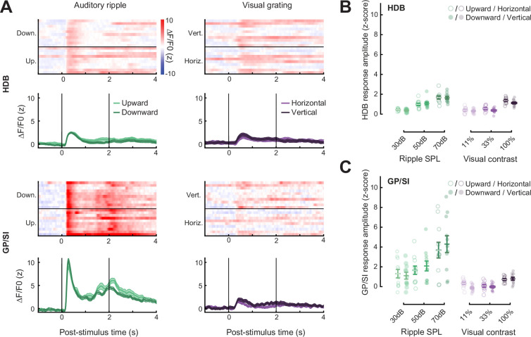
Figure 2u2014figure supplement 1.
Equivalent basal forebrain cholinergic neuron (BFCN) responses to varying directions of auditory and visual drifting gratings.
( A ) BFCN responses to auditory spectrotemporal ripples ( left column ) and visual gratings ( right column ) of varying direction are shown for an example mouse. Heatmaps depict fractional change val...
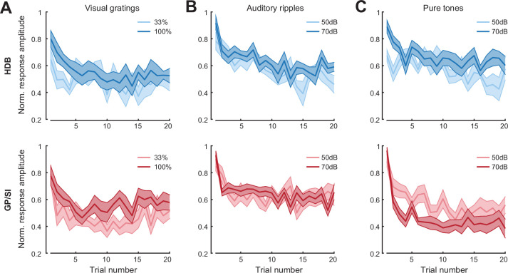
Figure 2u2014figure supplement 2.
Basal forebrain cholinergic neuron (BFCN) responses to unconditioned sensory cues rapidly habituate across stimulus type, modality, and intensity.
( A ) Mean u00b1 SEM normalized BFCN response to visual drifting gratings were significantly and equivalently reduced in horizontal limb of the diagonal band of Broca (HDB) ( top ) and globus pallidus...
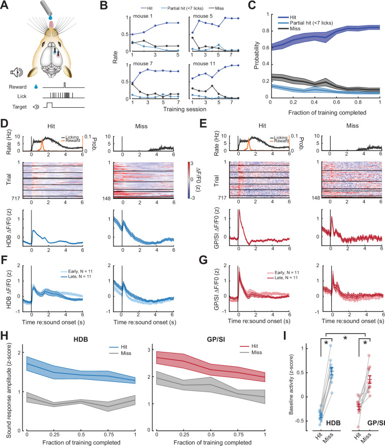
Figure 3.
Pre-stimulus cholinergic basal forebrain activity distinguishes behavioral hit and miss trials during an auditory detection task.
( A ) Mice were rewarded for producing a vigorous bout of licking (at least 7 licks in 2.8 s) shortly after a low-, mid-, or high-frequency tone. ( B ) Learning curves from four example mice that beca...
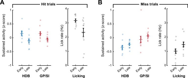
Figure 3u2014figure supplement 1.
Lick rates may account for subtle differences in sustained basal forebrain cholinergic neuron (BFCN) sustained activity across learning.
( A ) On hit trials, sustained BFCN activity (3u20136 s following the onset of the auditory cue) is greater in early training than later in the training period, but so is the lick rate measured during...
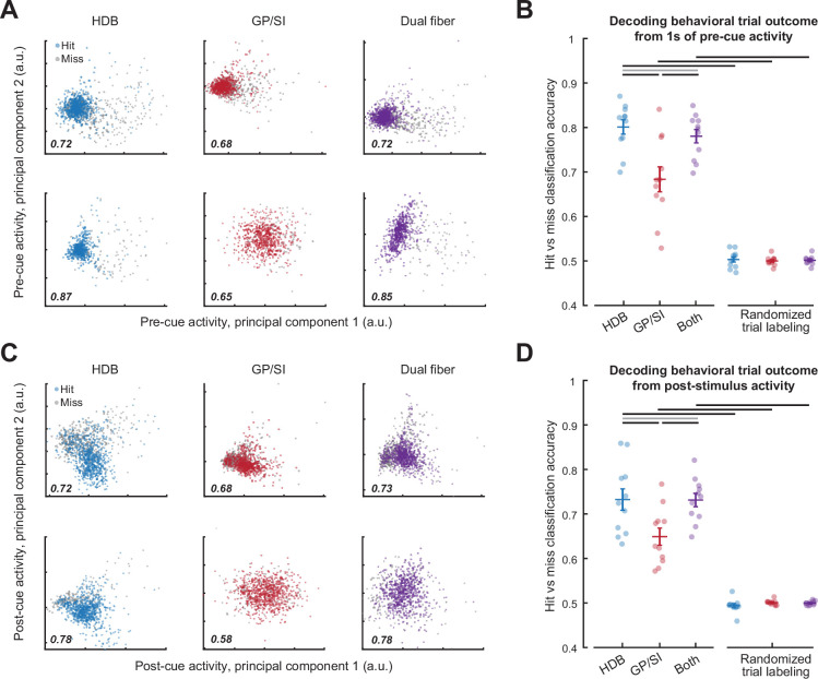
Figure 4.
Pre- and post-cue basal forebrain cholinergic neuron (BFCN) activity predicts behavioral accuracy.
( A ) Bulk BFCN activity measured 1 s prior to tone onset for two representative mice. Circles denote activity from individual hit and miss trials projected onto the first two principal components. A ...
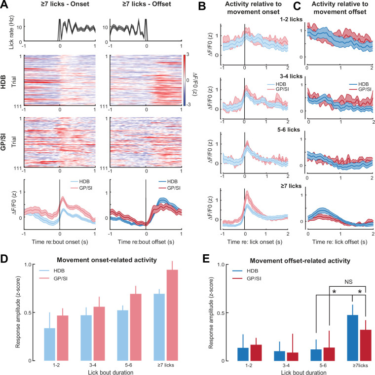
Figure 5.
Motor-related activation of the cholinergic basal forebrain.
( A ) Horizontal limb of the diagonal band of Broca (HDB) and globus pallidus and substantia innominata (GP/SI) activity from an example mouse related to the onset (left column) and offset (right colu...
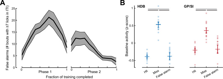
Figure 5u2014figure supplement 1.
False alarms were relatively uncommon and were not associated with elevated baseline basal forebrain cholinergic neuron (BFCN) activity.
( A ) Mean u00b1 SEM incidence of false alarm events during the inter-trial interval (ITI) period measured during Phase 1 (all frequencies rewarded) and Phase 2 (variable reinforcement outcome) of the...
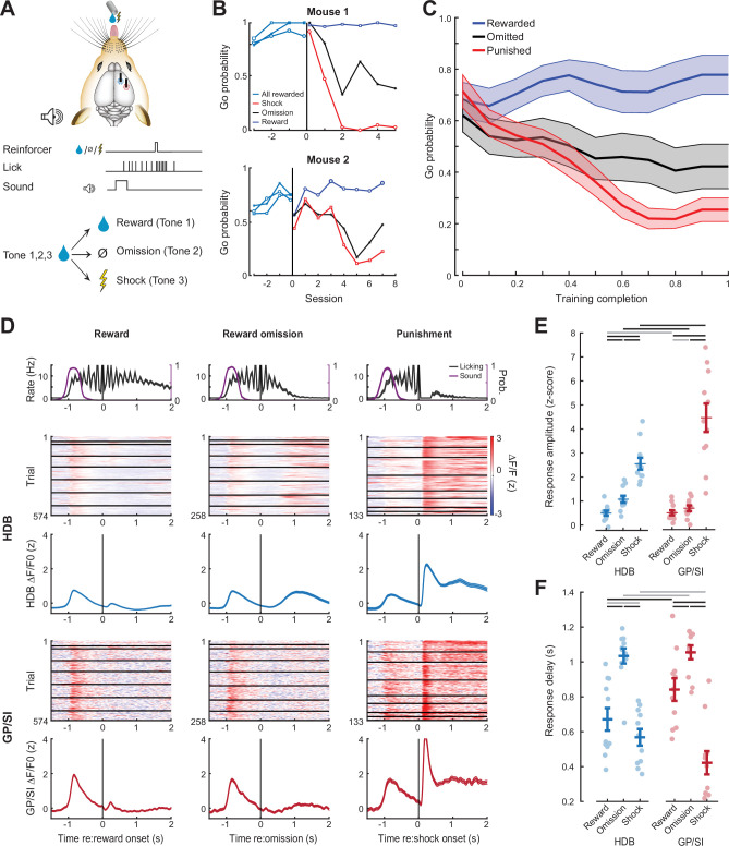
Figure 6.
Differential responses of horizontal limb of the diagonal band of Broca (HDB) and globus pallidus and substantia innominata (GP/SI) basal forebrain cholinergic neurons (BFCNs) to reward, punishment, and reward omission.
( A ) Once mice were reliably licking for reward following the onset of the low-, mid-, or high-frequency tone, the reinforcement outcome was changed such that u22657 licks in 2.8 s elicited a tongue ...
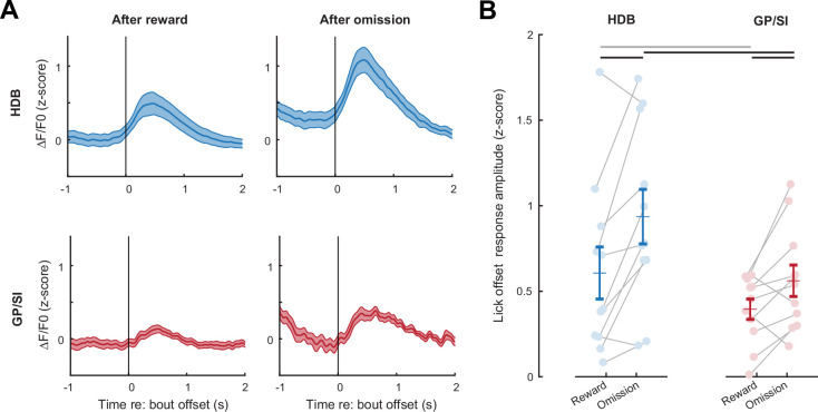
Figure 6u2014figure supplement 1.
Basal forebrain responses on omission trials reflect reinforcement prediction error, not a motor-related signal.
( A ) Mean u00b1 SEM tone-evoked GCaMP activity in horizontal limb of the diagonal band of Broca (HDB) and globus pallidus and substantia innominata (GP/SI) (N = 11 mice) relative to the offset of lic...
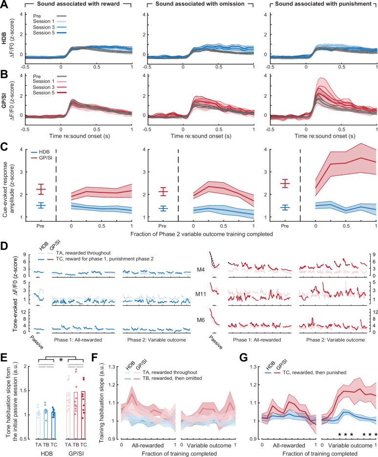
Figure 7.
Enhanced basal forebrain cholinergic neuron (BFCN) responses to punishment-predicting cues in globus pallidus and substantia innominata (GP/SI), not horizontal limb of the diagonal band of Broca (HDB).
( Au2013B ) Mean u00b1 SEM tone-evoked GCaMP activity in HDB (N = 11, A ) and GP/SI ( B ) for the tone frequency associated with reward (left column), reward omission (middle column), and punishment (...
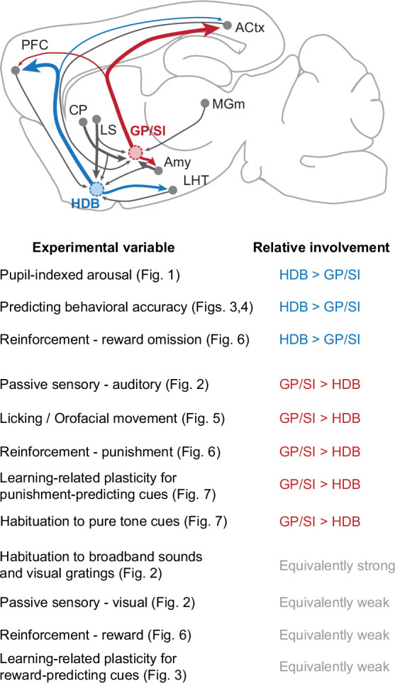
Figure 8.
Summary of functional specializations in the rostral and caudal basal forebrain.
A summary of the relative involvement of horizontal limb of the diagonal band of Broca (HDB) and globus pallidus and substantia innominata (GP/SI) across all experimental variables tested in this stud...
Author response image 1.
Figure images are served from the NIH/NLM PubMed Central Open Access Subset or Europe PMC; copyright remains with the publishers and authors.
💬 Discussion
0 commentsNo comments yet. Be the first to start a discussion!
Leave a Comment