Abstract
To move the body, the brain must precisely coordinate patterns of activity among diverse populations of motor neurons. Here, we use in vivo calcium imaging, electrophysiology, and behavior to understand how genetically-identified motor neurons control flexion of the fruit fly tibia. We find that leg motor neurons exhibit a coordinated gradient of anatomical, physiological, and functional properties. Large, fast motor neurons control high force, ballistic movements while small, slow motor neurons control low force, postural movements. Intermediate neurons fall between these two extremes. This hierarchical organization resembles the size principle, first proposed as a mechanism for establishing recruitment order among vertebrate motor neurons. Recordings in behaving flies confirmed that motor neurons are typically recruited in order from slow to fast. However, we also find that fast, intermediate, and slow motor neurons receive distinct proprioceptive feedback signals, suggesting that the size principle is not the only mechanism that dictates motor neuron recruitment. Overall, this work reveals the functional organization of the fly leg motor system and establishes Drosophila as a tractable system for investigating neural mechanisms of limb motor control. In the body, spindly nerve cells called motor neurons connect the brain to the muscles. Their role is to control movement, as they translate the electrical signals from the brain into instructions to the muscles. In humans, it takes over 150,000 motor neurons to control the movement of one leg; in contrast, fruit flies only need 50 neurons to operate a leg, despite also executing a variety of movements. Fruit flies are commonly used in laboratories to study an array of biological processes, yet little is known about how their motor neurons direct movements. In particular, it was unclear whether the same principles that control how muscles contract in mammals also applied in the tiny fruit fly. To begin investigating, Azevedo et al. mapped out the arrangement of motor neurons that control muscles in the fruit fly leg. As the leg moved, the activity of both the neurons and the muscles they controlled was recorded, as well as the force that had been generated. The experiments showed that each motor neuron controls a certain range of leg force and speed: some produced small, slow motion important for posture and dexterity, while others created large, fast movements essential to running or escape. In addition, the neurons activate in a particular order – cells that control slow movements fire first, and those that direct fast maneuvers later. These processes are also found in other organisms, but the difference is that flies have so few neurons, allowing scientists to reliably identify each motor neuron. Future experiments will therefore be able to test how flies recruit the right neurons to create specific movement sequences. Fruit flies are often used to research human illnesses that affect movement, such as motor neuron disease. A better understanding of the way their neural circuits coordinate the body could help reveal how these conditions emerge.
🔬 Techniques
🔭 Microscopes
🧬 Organisms
✨ Fluorophores
🧪 Sample Preparation
🔬 Cell Lines
🏭 Microscope Brands
🧪 Reagent Suppliers
💻 Software Details
💻 Code & Software
Official implementation of DeepLabCut: Markerless pose estimation of user-defined features with deep learning for all animals incl. humans
Fly sounds
Simple script to label imgXXX.png images for training sets for DLC
Interactively detect spikes in D mel data
Fly sounds
Analysis routines for data gathered with FlySound acquisition package
💾 Data Repositories
🏷️ Research Resource Identifiers (RRIDs)
Verified research resources used in this paper:
🏛️ Research Organizations (ROR)
Affiliated research institutions:
📋 Methods
Key resources table
Reagent type (species) or resource Designation Source or reference Identifiers Additional information Genetic reagent ( D. melanogaster ) ‘w[*]; P{w[+mC]=Mhc-GAL4.K}2’ Bloomington Drosophila Stock Center RRID: BDSC_55133 Genetic reagent ( D. melanogaster ) ‘P{y[+t7.7] w[+mC]=20XUAS-IVS-mCD8::GFP}attP2’ Bloomington Drosophila Stock Center RRID: BDSC_32194 Genetic reagent ( D. melanogaster ) ‘P{y[+t7.7] w[+mC]=GMR22A08-GAL4}attP2’ Bloomington Drosophila Stock Center RRID: BDSC_47902 Genetic reagent ( D. melanogaster ) ‘P{JFRC7-20XUAS-IVS-mCD8::GFP} attp40’ Other FBrf0212432 Barret Pfeiffer, Janelia Farm, HHMI Genetic reagent ( D. melanogaster ) ‘MHC-LexA’ Other Richard Mann, Columbia University Genetic reagent ( D. melanogaster ) ‘13XLexAop2-IVS-GCaMP6f-p10}su(Hw)attP5’ Bloomington Drosophila Stock Center RRID: BDSC_44277 Genetic reagent ( D. melanogaster ) ‘Berlin-K’ Bloomington Drosophila Stock Center RRID: BDSC_8522 Genetic reagent ( D. melanogaster ) ‘P{y[+t7.7] w[+mC]=GMR81A07-GAL4}attP2’ Bloomington Drosophila Stock Center RRID: BDSC_40100 Genetic reagent ( D. melanogaster ) ‘P{y[+t7.7] w[+mC]=GMR35 C09-GAL4}attP2’ Bloomington Drosophila Stock Center RRID: BDSC_49901 Genetic reagent ( D. melanogaster ) ‘10XUAS-syn21-Chrimson88-tDT3.1 (attP18)’ DOI: 10.1016/j.neuron.2017.03.010 Michael Reiser, Janelia Farm, HHMI Genetic reagent ( D. melanogaster ) ‘P{y[+t7.7] w[+mC]=20 XUAS-IVS-CsChrimson.mVenus}attP2’ Bloomington Drosophila Stock Center RRID: BDSC_55136 Genetic reagent ( D. melanogaster ) ‘iav-LexA’ Bloomington Drosophila Stock Center RRID: BDSC_52246 Genetic reagent ( D. melanogaster ) ‘13XLexAop2-IVS-Syn-21-Chrimson::tdTomato (attP2)’ DOI: 10.1038/nmeth.2836 Barret Pfeiffer, Janelia Farm, HHMI Genetic reagent ( D. melanogaster ) ‘P{y[+t7.7] w[+mC]=BDP-GAL4}attP2’ DOI: 10.7554/eLife.08758.027 Andrew Seeds, Steffi Hampel, UNIVERSITY OF PUERTO RICO Genetic reagent ( D. melanogaster ) ‘P{w[+mW.hs]=GawB}VGlut[OK371]’ Bloomington Drosophila Stock Center RRID: BDSC_26160 Antibody nc82 (mouse monoclonal) Developmental Studies Hybridoma Bank, RRID: AB_2314866 1:50 Chemical compound, drug MLA Tocris TOCRIS_1029 ‘1 μM methyllycaconitine citrate’ Software, algorithm MATLAB Mathworks RRID: SCR_001622 Software, algorithm DeepLabCut DOI: 10.1038/s41593-018-0209-y Mathis Lab, Rowland Institute, Harvard University https://github.com/AlexEMG/DeepLabCut Software, algorithm FIJI PMID: 22743772 RRID: SCR_002285 Software, algorithm Fictrac DOI: 10.1016/j.jneumeth.2014.01.010 Other Force probe fiber Proform CS2.5 AS This paper “PBT fiber from a synthetic paint brush, cut to have a spring constant = 0.22 N/m. Find at any Proform retailer, e.g. Amazon.com ’ Other Green CST DPSS laser, Besram Technology, Inc ‘532 nm’ Other Phalloidin ThermoFisherScientific FISHER: A22284 ‘633 nm, 1 unit per leg’ Other streptavidin-Alexa Fluor ThermoFisherScientific FISHER: S11226 ‘568 nm’ Fly husbandry Drosophila melanogaster were raised on cornmeal agar food on a 14 hr dark/10 hr light cycle at 25°C and 70% relative humidity. We used female flies, 1–4 days post eclosion, for all experiments except tethered behavior experiments. Both male and female dark-reared flies, between 2–10 days post-eclosion, were used for tethered walking behavior experiments. For experiments involving optogenetic reagents (Chrimson variants and gtACR1), adult flies were placed on cornmeal agar with all-trans-retinal (100 µL of 35 mM ATR in 95% EtOH, Santa Cruz Biotechnology) for 24 hr prior to the experiment. Vials were wrapped in foil to reduce optogenetic activation during development.
Show full methods section
Key resources table
Reagent type (species) or resource Designation Source or reference Identifiers Additional information Genetic reagent ( D. melanogaster ) ‘w[*]; P{w[+mC]=Mhc-GAL4.K}2’ Bloomington Drosophila Stock Center RRID: BDSC_55133 Genetic reagent ( D. melanogaster ) ‘P{y[+t7.7] w[+mC]=20XUAS-IVS-mCD8::GFP}attP2’ Bloomington Drosophila Stock Center RRID: BDSC_32194 Genetic reagent ( D. melanogaster ) ‘P{y[+t7.7] w[+mC]=GMR22A08-GAL4}attP2’ Bloomington Drosophila Stock Center RRID: BDSC_47902 Genetic reagent ( D. melanogaster ) ‘P{JFRC7-20XUAS-IVS-mCD8::GFP} attp40’ Other FBrf0212432 Barret Pfeiffer, Janelia Farm, HHMI Genetic reagent ( D. melanogaster ) ‘MHC-LexA’ Other Richard Mann, Columbia University Genetic reagent ( D. melanogaster ) ‘13XLexAop2-IVS-GCaMP6f-p10}su(Hw)attP5’ Bloomington Drosophila Stock Center RRID: BDSC_44277 Genetic reagent ( D. melanogaster ) ‘Berlin-K’ Bloomington Drosophila Stock Center RRID: BDSC_8522 Genetic reagent ( D. melanogaster ) ‘P{y[+t7.7] w[+mC]=GMR81A07-GAL4}attP2’ Bloomington Drosophila Stock Center RRID: BDSC_40100 Genetic reagent ( D. melanogaster ) ‘P{y[+t7.7] w[+mC]=GMR35 C09-GAL4}attP2’ Bloomington Drosophila Stock Center RRID: BDSC_49901 Genetic reagent ( D. melanogaster ) ‘10XUAS-syn21-Chrimson88-tDT3.1 (attP18)’ DOI: 10.1016/j.neuron.2017.03.010 Michael Reiser, Janelia Farm, HHMI Genetic reagent ( D. melanogaster ) ‘P{y[+t7.7] w[+mC]=20 XUAS-IVS-CsChrimson.mVenus}attP2’ Bloomington Drosophila Stock Center RRID: BDSC_55136 Genetic reagent ( D. melanogaster ) ‘iav-LexA’ Bloomington Drosophila Stock Center RRID: BDSC_52246 Genetic reagent ( D. melanogaster ) ‘13XLexAop2-IVS-Syn-21-Chrimson::tdTomato (attP2)’ DOI: 10.1038/nmeth.2836 Barret Pfeiffer, Janelia Farm, HHMI Genetic reagent ( D. melanogaster ) ‘P{y[+t7.7] w[+mC]=BDP-GAL4}attP2’ DOI: 10.7554/eLife.08758.027 Andrew Seeds, Steffi Hampel, UNIVERSITY OF PUERTO RICO Genetic reagent ( D. melanogaster ) ‘P{w[+mW.hs]=GawB}VGlut[OK371]’ Bloomington Drosophila Stock Center RRID: BDSC_26160 Antibody nc82 (mouse monoclonal) Developmental Studies Hybridoma Bank, RRID: AB_2314866 1:50 Chemical compound, drug MLA Tocris TOCRIS_1029 ‘1 μM methyllycaconitine citrate’ Software, algorithm MATLAB Mathworks RRID: SCR_001622 Software, algorithm DeepLabCut DOI: 10.1038/s41593-018-0209-y Mathis Lab, Rowland Institute, Harvard University https://github.com/AlexEMG/DeepLabCut Software, algorithm FIJI PMID: 22743772 RRID: SCR_002285 Software, algorithm Fictrac DOI: 10.1016/j.jneumeth.2014.01.010 Other Force probe fiber Proform CS2.5 AS This paper “PBT fiber from a synthetic paint brush, cut to have a spring constant = 0.22 N/m. Find at any Proform retailer, e.g. Amazon.com ’ Other Green CST DPSS laser, Besram Technology, Inc ‘532 nm’ Other Phalloidin ThermoFisherScientific FISHER: A22284 ‘633 nm, 1 unit per leg’ Other streptavidin-Alexa Fluor ThermoFisherScientific FISHER: S11226 ‘568 nm’ Fly husbandry Drosophila melanogaster were raised on cornmeal agar food on a 14 hr dark/10 hr light cycle at 25°C and 70% relative humidity. We used female flies, 1–4 days post eclosion, for all experiments except tethered behavior experiments. Both male and female dark-reared flies, between 2–10 days post-eclosion, were used for tethered walking behavior experiments. For experiments involving optogenetic reagents (Chrimson variants and gtACR1), adult flies were placed on cornmeal agar with all-trans-retinal (100 µL of 35 mM ATR in 95% EtOH, Santa Cruz Biotechnology) for 24 hr prior to the experiment. Vials were wrapped in foil to reduce optogenetic activation during development.
Electrophysiology and calcium imaging preparation
Flies were positioned in a custom steel holder as described in Tuthill and Wilson, 2016b , with modifications to allow us to image movement of the fly leg. Each fly was anesthetized on ice for two minutes, so that she could be positioned ventral side up with her head and thorax fixed in place with UV-cured glue. The front legs were glued to the horizontal top of the holder, the coxa aligned with the thorax, and the femur positioned at a right angle to the coxa and body axis. In this configuration, the fly could freely wave her tibia in an arc at an angle of ~50–65° to the top surface of the holder. The holder was placed in the imaging plane of a Sutter SOM moveable objective microscope. All recordings were performed in extracellular fly saline (recipe below) at room temperature. We used a water immersion 40X objective (Nikon) for patch-clamping and a 5X air objective (Nikon) to view the fly’s right front femur and tibia through the saline during spontaneous movements of the leg. Videos of the preparation were acquired at 170 Hz through the 5X objective with a Basler acA1300-200um machine vision camera. Custom acquisition code written in MATLAB ( Azevedo, 2020a ; copy archived at https://github.com/elifesciences-publications/FlySound ) controlled generation and acquisition of digital and analog signals through a DAQ (National Instruments). Input signals were digitized at 50 kHz.
Force measurement and spring constant calibration
To measure forces produced by leg movements, we imaged the position of a flexible ‘force probe’ as the fly pulled against it. The force probe was a PBT filament fiber from a synthetic paint brush (Proform CS2.5 AS), threaded through the end of a glass micropipette (1.5 mm OD, 1.1 mm ID, WPI). To create a force probe, UV-cured glue (KOA 300, KEMXERT) was sucked up into the micropipette, the fiber was threaded into the glue, leaving 1–2 cm protruding out from the tip of the glass, and the glue was cured. The micropipette allowed us to mount the force probe in a custom holder and to couple it to a micromanipulator (Sutter MP-285). Videos of the force probe were acquired at 170 Hz through the 5X objective with a Basler acA1300-200um machine vision camera. One pixel equaled 1.03 μm 2 . We wrote custom machine vision code that detects the position of the force probe in each frame of the video by 1) allowing the user to draw a line along the probe in the video, 2) rotate the image of the probe perpendicular to the line, 3) average down the rows of the rotated image to get a single intensity profile, with a peak at the probe’s location, and then 4) find the center of mass of the intensity peak,±FWHM above baseline. A similar technique employing a probe to measure force has been used in Drosophila in previous studies ( Elliott and Sparrow, 2012 ). At steady state, the position of the force probe was related to the force through a spring constant, k, F = -kx ( Figure 1—figure supplement 2 ). We measured the spring constant by positioning the force probe over an analytical balance. A glass coverslip was oriented vertically on edge in a piece of wax on the balance, and the tip of the force probe was positioned at the top edge of the coverslip. We then moved the micromanipulator to different positions. The ‘mass’ of the force probe was multiplied by gravity to give the force at that position. We then fit a linear relationship between force and position to measure the spring constant ( Figure 1—figure supplement 2A ). The force probe we used for experiments in this study had a spring constant of k = 0.2234 µN/µm and protruded approximately 1.5 cm past the end of the micropipette. The force probe was not only a spring. It also had mass and was placed in saline, so inertia ( m ) and drag ( c ) affected its dynamics: F = m d 2 x / d t 2 + c d x / d t + k x . To measure these properties, we ‘flicked’ the force probe by moving it to different positions with a glass micropipette, abruptly letting go, and allowing the probe to relax back to rest ( Figure 1—figure supplement 2B ). We imaged the position of the probe at 1.2 kHz with a restricted region of interest, and extracted dynamical parameters m = 0.1702 mg and c = 0.1377 kg/s. While not zero, the effective mass and drag were negligible ( Figure 1—figure supplement 2C ). The probe was slightly under-damped with a relaxation time constant of 2.5 ms and oscillation period of 5.8 ms, such that when imaging spontaneous movements at 170 Hz, the probe would effectively come to rest within one frame. The relaxation time constant was much faster than the fly’s spontaneous movements, even when the fly was attempting to let go of the force probe. In Figure 4D–F , we calculate force by including drag and inertia, but in other figures we report leg displacement and the approximation of force, assuming that drag and inertia are negligible. We easily captured the lateral movement of the force probe across the frame but avoided estimating the vertical movement as the fly pulled the probe closer to its leg. As a result, the displacement (and thus the force) measured by the probe in Figures 1 , 5 may be slightly underestimated. Mechanical stimulation of the leg To move the leg and passively stimulate proprioceptive feedback, we mounted the force probe perpendicularly on a piezoelectric actuator with a 60 μm travel range (Physik Instrumente). The axial position of the probe was controlled by an amplifier (Physik), with voltage commands generated in MATLAB and delivered through the DAQ board (National Instruments). The output of the actuator’s strain gauge was used to control the position of the actuator through closed-loop feedback. The strain gauge sensor output was sampled at 50 kHz. The probe tip was positioned near the end of the tibia, giving a lever arm of 417 ± 7 (s.d.) μm across flies (n = 8). We then moved the tibia through its range of motion until it was approximately at 90° to the femur. To measure the effect of leg angle on the amplitude of sensory feedback, we then moved the probe to a range of axial positions (−150 μm = −21°, −75 μm = −10°, 75 μm = 10° and 150 μm = 21°, negative direction is extension) and repeated the stimuli ( Figure 6—figure supplement 1 ). We delivered ramp stimuli that moved the leg 60 μm (8°) with varying speeds, in both flexion (+) and extension (-) directions. We measured the actual speed of step stimuli by finding the maximum derivative of the strain gauge signal during the step onset. The range of angular velocities produced by the probe span the range shown to activate position- and velocity-sensitive femoral chordotonal neurons in the femur ( Mamiya et al., 2018 ). Though the force probe was flexible, when we imaged the displacement of the force probe we saw that the probe tip matched the strain gauge feedback (errors < 5%), suggesting that passive or muscle forces did not impact these small stimuli. To generate larger, faster movements than we could deliver with the probe, we whacked the leg by flicking the probe, similar to how we calibrated the probe dynamics ( Figure 6—figure supplement 1 ).
Leg tracking
In trials where the fly was free to wave its leg rather than pull on the force probe, we tracked the leg using DeepLabCut ( Mathis et al., 2018 ). For a training set, we labeled the tibia position for ~45 frames for three different videos from each fly using custom labeling code ( Azevedo, 2020b ; copy archived at https://github.com/elifesciences-publications/LabelSelectedFramesForDLC ) . We labeled six points on the stationary femur, six points on the tibia ( Figure 1—figure supplement 1B ), as well as prominent bright objects that would otherwise often be falsely identified as part of the legs, such as the EMG electrode, the force probe, and several specular creases in the steel holder. The resnet50 network used in DeepLabCut served as the starting point for training, but as we added more flies to the training set, we initiated further training from the previously trained network. We found that the networks failed to generalize across flies but that ~150 labeled frames were sufficient to ensure >99% accuracy on other frames for that fly ( Figure 1—figure supplement 1B ). In post-processing, we measured the distribution of pairwise nearest neighbor distances between the six detected tibia points and assumed that outliers indicated that a point was poorly identified. If only a single point was misidentified (~0.7%), we filled in the point with random draws from the nearest-neighbor pairwise distance distributions. The network misidentified more than one point 0.2% of the time, typically when the fly moved its leg particularly quickly, causing the image to blur. We excluded such frames. We median-filtered the x, y coordinates across video frames, and found the centroid of the six points, approximately the middle of the tibia. The centroid points traced out an ellipse that was the projection of the circular arc of the leg in the plane of the camera. Fitting an ellipse to the centroids allowed us to calculate the azimuthal angle of the leg arc (~50–65°) and the real angle between the stationary femur and the moving leg. We then used the real angle of the leg to detect when the leg was extended (>120°) or flexed (40% of the pixels in a cluster, that cluster intensity for that frame was excluded from the analysis. The time constant of the calcium indicator was slower than the fly’s movements, such that fluorescence built up over subsequent contractions. Thus, pixel intensity (ΔF/F) was not directly related to contraction of the muscle. We took positive increases in cluster intensity to indicate muscle activation, i.e. neural activity. We applied a Sovitzky-Golay filter to interpolate cluster calcium signals (50 Hz) to the leg movements (170 Hz), which also computed the time-derivative of the local spline for each cluster (sgolay_t function in MATLAB, by Tiago Ramos, N = 7, F = 9). GCaMP6f decay was slow relative to leg movements ( Figure 1E and Figure 1—figure supplement 1E ), so negative derivatives reflected noise in the cluster fluorescence. We used this estimate of the noise (two standard deviations) to threshold the positive cluster derivatives, and thus find cluster ‘activations’. Surprisingly, we did not identify any clusters that increased their calcium activity during tibia extension. Flies occasionally held their legs extended ( Video 1 ), at which point we expected to see some clusters increase fluorescence ( Figure 1—figure supplement 1D–E ). On average, the leg musculature was dim during these periods Figure 1—figure supplement 1E ), whereas the fluorescence of superficial flexors muscle fibers could increase more than six-fold during flexion events. Diffuse emission from the bright and slowly fading flexors may have obscured small increases in extensor fluorescence. We still found it curious that contractions of extensors did not produce brighter events. We speculate that calcium influx and contractile forces may be larger in flexor muscles than extensors because flies use flexion of the forelimb tibia to support their weight, to hold onto the substrate, and to pull their body during walking, whereas extensors generally lift up unloaded limbs when swinging them forward.
Whole-cell patch clamp electrophysiology
To perform whole-cell patch clamp recordings, we first covered the fly in a drop of extracellular saline and dissected a window in the ventral cuticle of the thorax to expose the VNC. The perineural sheath surrounding the VNC was ruptured manually with forceps, near the midline, anterior to the T1 neuromeres. We first used a large bore cleaning pipette (~7–10 μm opening) to remove debris and gently blow cell bodies apart, clearing a path from the ruptured hole in the sheath to the targeted motor neuron soma. The recording chamber was then transferred to the microscope and perfused with saline at a rate of 2–3 mL/min. The extracellular saline solution was composed of (in mM) 103 NaCl, 3 KCl, 5 TES, eight trehalose, 10 glucose, 26 NaHCO3, 1 NaH2PO4, 4 MgCl2, 1.5 CaCl2. Saline pH was adjusted to 7.2 and osmolality was adjusted to 270–275 mOsm. Saline was bubbled with 95% O2/5% CO2. Whole-cell patch pipettes were pulled with a P-97 linear puller (Sutter Instruments) from borosilicate glass (OD 1.5 mm, ID 0.86 mm) to have approximately 5 MOhm resistance. Pipettes were then pressure-polished ( Goodman and Lockery, 2000 ) using a microforge equipped with a 100X inverted objective (ALA Scientific Instruments). Polished pipettes had resistances of approximately 12 MOhms. The polished surface allowed for high seal resistances (>50 GΩ) to limit the impact of seal conductance on V rest (200 pA from the fast motor neuron. Fast neuron units were by far the largest amplitude events in the femur. When the electrode was placed in the proximal part of the femur, near the terminal bristle, the spikes from the fast neuron tended to be smaller but still identifiable. We could not unambiguously detect EMG units associated with Flexor 3 in Figure 1 . We ran our spike detection routines (see below) on EMG records only in cases where they could be clearly identified or when EMG spikes aligned with the somatic spikes.
Optogenetic activation of leg motor neurons during electrophysiology
To measure force production as a function of motor neuron activity, we drove the expression of CsChrimson ( Klapoetke et al., 2014 ) with 81A07-Gal4, and the expression of Chrimson88 ( Strother et al., 2017 ) with 22A08-Gal4. CsChrimson expression in 22A08-Gal4 prevented straightening of the wings and caused the front legs to be bent midway through each segment. We drove expression of Chrimson ( Klapoetke et al., 2014 ) in sensory neurons with iav- LexA. We activated Chrimson by placing a fiber-coupled cannula (105 μm diameter, Thorlabs) next to the ventral window in the cuticle and illuminating the T1 neuropil with a 625 nm LED (Thorlabs). We used short flashes of 10 or 20 ms to activate neurons, increasing intensity by increasing the voltage supplied to the LED driver (Thorlabs). We measured the power output of the LED for each voltage we used.
Spike detection from whole-cell recordings and EMG recordings
To detect spikes in current clamp recordings of membrane potential, we applied the following analysis steps to our electrophysiology traces (digitized at 50 kHz): 1) filter, 2) identify events with large peaks above a threshold, 3) compare the shape of the filtered events to a template (distance metric), 4) threshold events based both on the shape and on the amplitude of the unfiltered spike. The parameter space for each of these steps was explored in an interactive spike detection interface ( Azevedo, 2020c ; copy archived at https://github.com/elifesciences-publications/spikeDetection ) . We high-pass filtered the first derivative of each trace with a 3-pole Butterworth filter with a cutoff at 209 Hz, a low-pass filter with a 3-pole Butterworth filter with a 898 Hz cutoff. Empirically derived, this procedure resulted in a large positive peak associated with the rapid reversal of the membrane potential at the top of a spike. Events were identified by threshold crossing. Thresholds were in the range of 2–10 *10^−5 mV/s. The threshold was set as low as possible to reject baseline noise. Changes in membrane voltage associated with current injection and large secondary peaks associated with the filtered spike waveform oscillations often passed above threshold. Events that passed threshold were then compared with a template using a dynamic time warping procedure over a 251 sample window centered on the event. The template was calculated for each cell, and though the amplitude varied with spike amplitude, the template time course (shape) was generally similar across cells and genotypes. We then calculated the amplitude of the voltage fluctuation in the raw record associated with each event. Thus, each detected peak in the filtered data had a shape metric value and a spike amplitude. Events with both a similar shape (i.e. time course) as the template and a large amplitudes were identified as spikes. We inspected records by eye to reject occasional false positives, such as changes in membrane voltage caused by current injection. The algorithm was generally effective once the parameters were tuned for each cell. However, two cases typically caused spikes to become very difficult to unambiguously identify in slow motor neurons. First, during large current injections and the resulting depolarization, the spikes became very small and difficult to identify ( Figure 4 ). High frequency spikes were clear in the raw voltage, and the leg moved, so we do not believe the neurons entered depolarization block. In such cases we hand tuned the parameters and inspected the identified spikes by eye to estimate the spike rate. Second, prolonged self-generated flexion could also depolarize slow motor neurons to the point that spike detection was difficult, we speculate because of large synaptic conductances that decreased input resistance. By contrast, spike detection worked perfectly during high spike rates evoked by sensory feedback ( Figure 6 ). Since we were interested in measuring spike latencies and conduction velocities, we calculated the second derivative of the raw voltage trace, smoothed over five samples, for each identified spike. We found the peak of the second derivative, using that point as the onset/acceleration of the spike. We used the same algorithm to detect spikes from EMG current records, with different thresholding parameters in Step four for each recording due to the variability in EMG event size.
Immunohistochemistry
After a whole-cell motor neuron recording, we dissected the VNC but left the legs and head attached. We placed the tissue in 4% paraformaldehyde in phosphate-buffered saline (PBS) for 20 min, then separated and retained the VNC and the right leg with the filled motor neuron. The VNC tissue was washed in PBST (PBS + Triton, 0.2% w/w), placed in blocking solution (PBST + 5% normal goat serum) for 20 min, and then placed for 24 hr in blocking solution containing a primary antibody for neuropil counterstain (1:50 mouse anti-Bruchpilot, Developmental Studies Hybridoma Bank, nc82 s) and a streptavidin-Alexa Fluor conjugate to label the neurobiotin-filled motor neuron (Invitrogen). We washed the tissue again in PBST, and then placed the VNC in blocking solution containing secondary antibodies for 24 hr (1:250 goat anti-mouse Alexa Fluor conjugate from Invitrogen; streptavidin-Alexa Fluor). The leg was first incubated in blocking solution, like the VNC. Then it was placed in PBST containing 0.01% sodium azide (Thermo Fisher), 1 unit of phalloidin (Thermo Fisher) and the streptavidin-Alexa Fluor, and allowed to incubate for two weeks at 4°C, with occasional nutation. Following staining, the tissue was mounted in Vectashield (Vector Labs) and imaged on a Zeiss 510 confocal microscope (Zeiss). Cells were traced in FIJI ( Rueden et al., 2017 ; Schindelin et al., 2012 ), using the Simple Neurite Tracing plug-in ( Longair et al., 2011 ). Images in Figure 2 show the results of the filling function in the FIJI plug-in. In some cases, the neuropil counterstain (anti-Bruchpilot) was omitted and the native autofluorescence of the tissue (along with nonspecific binding of streptavidin and GFP fluorescence) was used as reference. To quantify morphology ( Figure 3 ), we measured the soma diameter, the width of the neurite entering the neuropil, and the width of the axon, as close to the exit of the neuropil as possible. We made two measurements for each image and location and averaged the values. Fly preparation for walking experiments Fly wings were clipped under cold anesthesia (3 mm/s) in the half second following laser stimulation. We noticed that the laser stimulus caused the empty Gal4 flies (BDP-Gal4) to decrease their walking speed slightly, likely because the flies could see the stimulus. This was particularly noticeable when we first used a fiber-coupled LED with a 105 µm diameter cannula. This prompted us to focus the laser on the fly’s left leg in order to further reduce the spot size and minimize the behavioral artifact. Even so, the optogenetic stimulus increased the probability that stationary flies would start walking ( Figure 7H ). To control for this effect, we compared the change in speed in motor neuron lines for each stimulus duration, to the change in speed in the control empty Gal4 flies (see statistical analysis below). In no-light trials, walking initiation ( Figure 7H , black and gray bars) and changes in speed ( Figure 7E , black traces) did not vary across different genotypes, although baseline walking speed varied slightly across the different lines.
Statistical analyses
For electrophysiology and calcium imaging results in Figures 1 – 6 , no statistical tests were performed a priori to decide upon sample sizes, but sample sizes are consistent with conventions in the field. Unless otherwise noted, we used the non-parametric Mann-Whitney-Wilcoxon rank-sum test to compare two populations (e.g. Figure 4 ) and 2-way ANOVA with Tukey-Kramer corrections for multiple comparisons across three populations (e.g. Figure 3 ). To compare changes in fluorescence across multiple clusters and extension vs flexion ( Figure 1 ), we used a 2-way ANOVA modeling an interaction between clusters and flexion vs. extension, with Tukey-Kramer corrections for multiple comparisons. To compare cluster ΔF/F of multiple clusters ( Figure 1—figure supplement 1 ), we used a 2-way ANOVA with Tukey-Kramer corrections for multiple comparisons. All statistical tests were performed with custom code in MATLAB. For fly walking behavior in Figure 7 , we used bootstrap simulations with 10,000 random draws to compare both the likelihood of stationary flies to start walking, as well as changes in walking speed ( Saravanan et al., 2019 ). Stationary trials were assigned a binary value to indicate that the fly began walking (1) or not (0). For a given stimulus duration and optogenetic condition (Chrimson or gtACR), the binary values for the empty Gal4 control flies and a motor neuron line were combined and then drawn randomly with replacement in proportion to the number of trials for each genotype. As a metric, we measured the difference in the fraction of flies that began walking. The p-value was the fraction of instances in which the randomly drawn distribution produced a value of our metric more extreme then we saw in the data (two-tailed) ( Figure 7H ). For trials in which the fly was already walking at the onset of the laser stimulus ( Walking trials, Figure 7E ), we compared the relative change in speed following the stimulus for a given motor neuron line to the empty Gal4 line. We randomly assigned trials to each genotype and calculated the average speed change as above. We used the Benjamini-Hochberg procedure to calculate the false-discovery-rate for either activation or silencing. Table of genotypes Figure 1A W[*]; P{w[+mC]=Mhc-GAL4.K}2, P{y[+t7.7] w[+mC]=20XUAS-IVS-mCD8::GFP}attP2 Figure 1B w[1118]; P{JFRC7-20XUAS-IVS-mCD8::GFP} attp40/+; P{y[+t7.7] w[+mC]=GMR22A08-GAL4}attP2/+ Figure 1C–I w[1118]; MHC-LexA,w[13XLexAop2-IVS-GCaMP6f-p10}su(Hw)attP5/Berlin WT; +/Berlin WT; Figure 2 w[1118]; P{JFRC7-20XUAS-IVS-mCD8::GFP} attp40/+; P{y[+t7.7] w[+mC]=GMR81A07-GAL4}attP2/+ w[1118]; P{JFRC7-20XUAS-IVS-mCD8::GFP} attp40/+; P{y[+t7.7] w[+mC]=GMR22A08-GAL4}attP2/+ w[1118]; P{JFRC7-20XUAS-IVS-mCD8::GFP} attp40/+; P{y[+t7.7] w[+mC]=GMR35 C09-GAL4}attP2/+ Figure 3 w[1118]; P{JFRC7-20XUAS-IVS-mCD8::GFP} attp40/+; P{y[+t7.7] w[+mC]=GMR81A07-GAL4}attP2/+ w[1118]; P{JFRC7-20XUAS-IVS-mCD8::GFP} attp40/+; P{y[+t7.7] w[+mC]=GMR22A08-GAL4}attP2/+ w[1118]; P{JFRC7-20XUAS-IVS-mCD8::GFP} attp40/+; P{y[+t7.7] w[+mC]=GMR35 C09-GAL4}attP2/+ Figure 4 w[1118]; P{JFRC7-20XUAS-IVS-mCD8::GFP} attp40/+; P{y[+t7.7] w[+mC]=GMR81A07-GAL4}attP2/P{y[+t7.7] w[+mC]=20 XUAS-IVS-CsChrimson.mVenus}attP2 w[1118], 10XUAS-syn21-Chrimson88-tDT3.1 (attP18); P{JFRC7-20XUAS-IVS-mCD8::GFP} attp40/+; P{y[+t7.7] w[+mC]=GMR22A08-GAL4}attP2/w[1118]; P{JFRC7-20XUAS-IVS-mCD8::GFP} attp40/+; P{y[+t7.7] w[+mC]=GMR35 C09-GAL4}attP2/+ Figure 5 w[1118]; P{JFRC7-20XUAS-IVS-mCD8::GFP} attp40/+; P{y[+t7.7] w[+mC]=GMR81A07-GAL4}attP2/+ w[1118]; P{JFRC7-20XUAS-IVS-mCD8::GFP} attp40/+; P{y[+t7.7] w[+mC]=GMR22A08-GAL4}attP2/+ w[1118]; P{JFRC7-20XUAS-IVS-mCD8::GFP} attp40/+; P{y[+t7.7] w[+mC]=GMR35 C09-GAL4}attP2/+ Figure 6A–E w[1118]; P{JFRC7-20XUAS-IVS-mCD8::GFP} attp40/+; P{y[+t7.7] w[+mC]=GMR81A07-GAL4}attP2/+ w[1118]; P{JFRC7-20XUAS-IVS-mCD8::GFP} attp40/+; P{y[+t7.7] w[+mC]=GMR22A08-GAL4}attP2/+ w[1118]; P{JFRC7-20XUAS-IVS-mCD8::GFP} attp40/+; P{y[+t7.7] w[+mC]=GMR35 C09-GAL4}attP2/+ Figure 6G–H w[1118]; P{JFRC7-20XUAS-IVS-mCD8::GFP} attp40/iav-LexA; P{y[+t7.7] w[+mC]=GMR81A07-GAL4}attP2/13XLexAop2-IVS-Syn-21-Chrimson::tdTomato (attP2) w[1118]; P{JFRC7-20XUAS-IVS-mCD8::GFP} attp40/iav-LexA; P{y[+t7.7] w[+mC]=GMR22A08-GAL4}attP2/13XLexAop2-IVS-Syn-21-Chrimson::tdTomato (attP2) w[1118]; P{JFRC7-20XUAS-IVS-mCD8::GFP} attp40/iav-LexA; P{y[+t7.7] w[+mC]=GMR35 C09-GAL4}attP2/13XLexAop2-IVS-Syn-21-Chrimson::tdTomato (attP2) Figure 7 w[1118]; +/+; P{y[+t7.7] w[+mC]=GMR81A07-GAL4}attP2/P{y[+t7.7] w[+mC]=20 XUAS-IVS-CsChrimson.mVenus}attP2 w[1118]; +/+; P{y[+t7.7] w[+mC]=GMR35 C09-GAL4}attP2/P{y[+t7.7] w[+mC]=20 XUAS-IVS-CsChrimson.mVenus}attP2 w[1118]; +/+; P{y[+t7.7] w[+mC]=GMR22A08-GAL4}attP2/P{y[+t7.7] w[+mC]=20 XUAS-IVS-CsChrimson.mVenus}attP2 w[1118]; +/+; P{y[+t7.7] w[+mC]=BDP-GAL4}attP2/P{y[+t7.7] w[+mC]=20 XUAS-IVS-CsChrimson.mVenus}attP2 w[1118]; +/+; P{y[+t7.7] w[+mC]=GMR81A07-GAL4}attP2/P{y[+t7.7] w[+mC]=20 XUAS-IVS- gtACR1}attP2 w[1118]; +/+; P{y[+t7.7] w[+mC]=GMR35 C09-GAL4}attP2/P{y[+t7.7] w[+mC]=20XUAS-IVS-gtACR1}attP2 w[1118]; +/+; P{y[+t7.7] w[+mC]=GMR22A08-GAL4}attP2/P{y[+t7.7] w[+mC]=20 XUAS-IVS- gtACR1}attP2 w[1118]; +/+; P{y[+t7.7] w[+mC]=BDP-GAL4}attP2/P{y[+t7.7] w[+mC]=20 XUAS-IVS- gtACR1}attP2 w[1118]; P{w[+mW.hs]=GawB}VGlut[OK371]/+; +/P{y[+t7.7] w[+mC]=20 XUAS-IVS- gtACR1}attP2 Data and software availability Data will be made available from the authors website. Acquisition code is available at https://github.com/tony-azevedo/FlySound . Analysis code is available at https://github.com/tony-azevedo/FlyAnalysis .
Additional files Transparent reporting form
📊 Figures
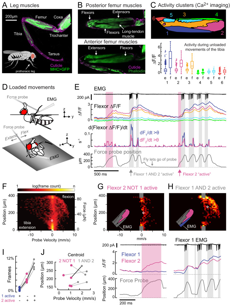
Figure 1.
Functional organization and recruitment order among muscles controlling the Drosophila leg.
( A )u00a0Muscles of the right prothoracic leg of a female Drosophila ( MHC-LexA; 20XLexAop-GFP ). ( B ) Muscles controlling tibia movement in the fly femur. Top and bottom are confocal sections throu...
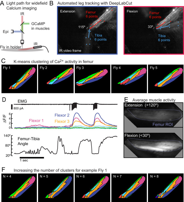
Figure 1u2014figure supplement 1.
Wide-field calcium imaging of muscles in the femur.
( A )u00a0Schematic of light path for widefield calcium imaging of femur muscles. Infrared illumination is used to track leg movement. GCaMP emission is reflected by a longpass dichroic mirror to a se...
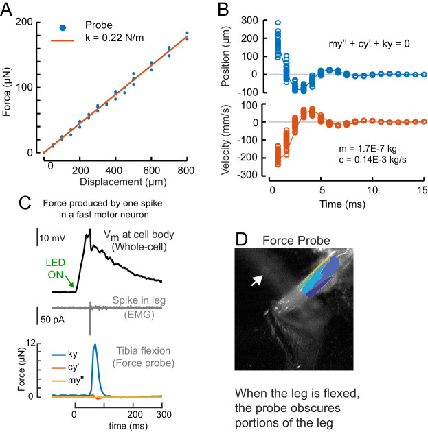
Figure 1u2014figure supplement 2.
Calibration of the force probe dynamic properties.
( A )u00a0The force probe tip was positioned over an analytical balance, and the base of the force probe was displaced. The weight (force) at each displacement is shown in blue, the linear fit is show...
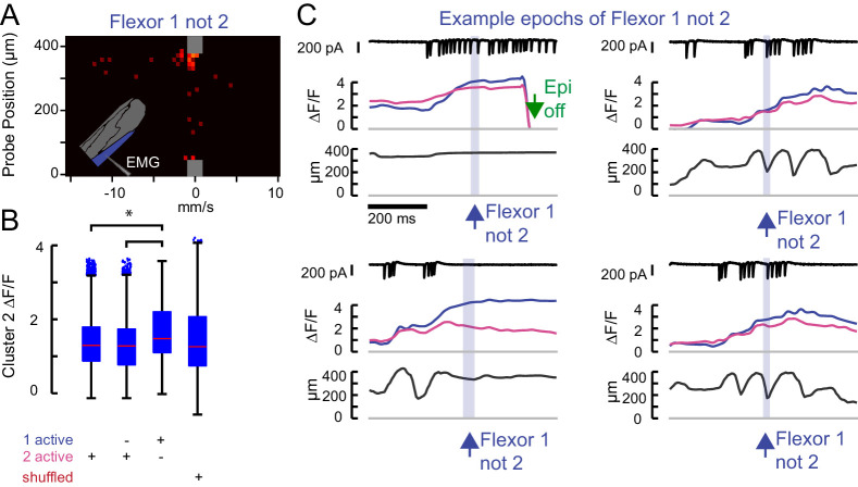
Figure 1u2014figure supplement 3.
Flexor 2 signal is high whenever Flexor 1u00a0isu00a0active.
( A )u00a0The force probe histogram for frames when only Flexor 1 was active, scaled according to Figure 1H . ( B ) Flexor 2 u0394F/F for all frames across Nu00a0=u00a05 flies in which 1) Flexor 2 is ...

Figure 1u2014figure supplement 4.
GFP control for k-means clustering of calcium activity.
( A )u00a0K-means clustering of GFP expression in muscles during spontaneous movements. Clusters were noisy, interleaved and dispersed. In this case, the fly pulled on the probe and the clusters are s...
Video 1.
Calcium imaging of femur muscles.
The video (1) illustrates the arrangement of musculature controlling the flyu2019s tibia; (2) schematizes the position of a restrained fly relative to the force probe fiber, together with wide-field c...
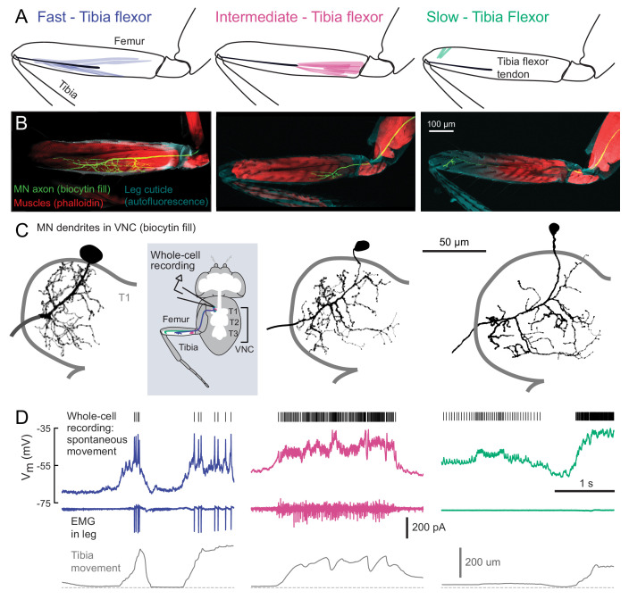
Figure 2.
Motor neurons controlling tibia flexion.
( A )u00a0Schematic of the muscle fibers innervated by motor neurons labeled by the following Gal4 lines: left: R81A07-Gal4 , center: R22A08-Gal4 , and right: R35C09-Gal4 . ( B ) Biocytin fills of leg...
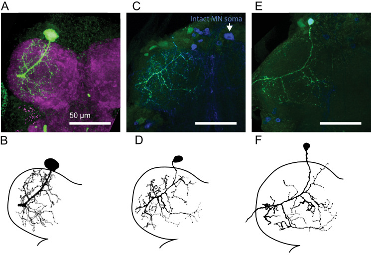
Figure 2u2014figure supplement 1.
Central anatomy of flexor motor neurons.
( A )u00a0Maximum intensity projections of fast flexor motor neuron fill (green, neurobiotin). In magenta is the neuropil (nc82). ( B ) Traced neuron from A ), using the simple neurite tracer plugin i...
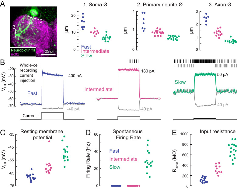
Figure 3.
A gradient of intrinsic properties among tibia flexor motor neurons.
( A )u00a0Left) Maximum intensity projection of a Neurobiotin fill (green) of the fast tibia flexor motor neuron, with nc82 counterstain. Right) Diameters of identified neuron 1) somas, 2) primary neu...
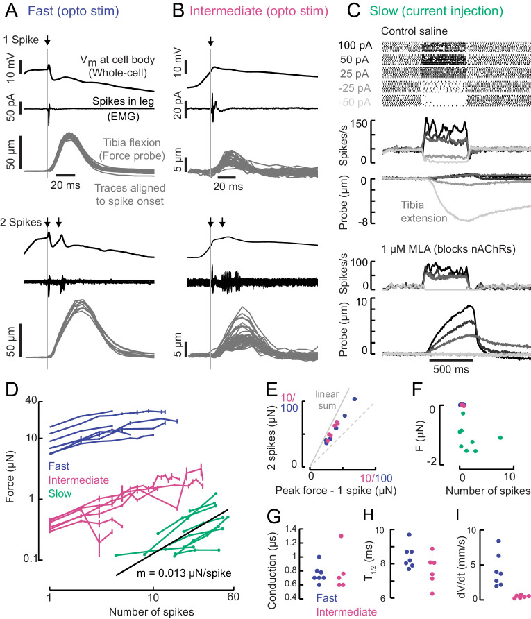
Figure 4.
A gradient of force production among tibia flexor motor neurons.
( A )u00a0Optogenetic activation of a fast flexor motor neuron expressing CsChrimson (50 ms flash from a 625 nm LED,~2 mW/mm 2 ). Traces show average membrane potential for trials with one (top) and t...
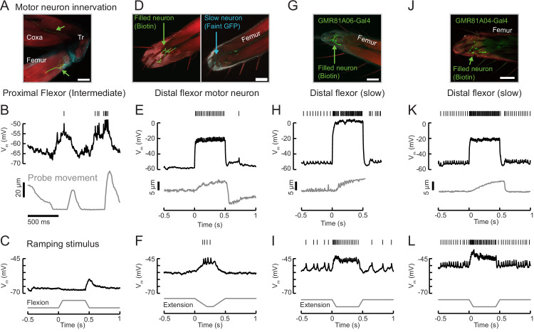
Figure 4u2014figure supplement 1.
Example recordings from other tibia flexor neurons.
( A )u00a0Confocal image of an intermediate flexor motor neuron axon (neurobiotin fill is shown in green; red is phalloidin) from UAS-GFP;R81A06-Gal4 . The filled neuron targets the proximal femur. Sc...
Video 2.
Motor neuron electrophysiology, force production, and tibia movement.
Theu00a0video introduces 1)u00a0the dendritic morphology and axon projection of the three neurons we studied: fast, intermediate and slow; 2) shows video of individual trials from a fast neuron in whi...
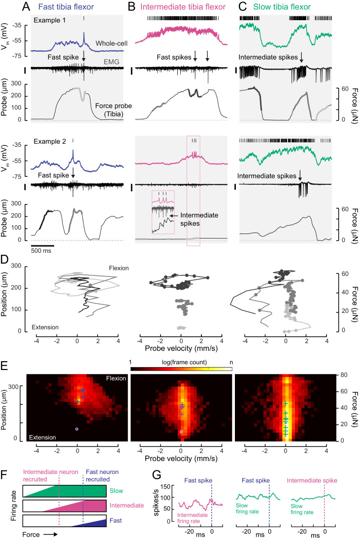
Figure 5.
Motor neurons are recruited in a specific order across different motor regimes.
( A )u00a0Membrane potential, EMG, and probe movement, for two example epochs of spontaneous leg movement during a whole-cell recording of the fast motor neuron. Highlighted events are plotted in D. T...
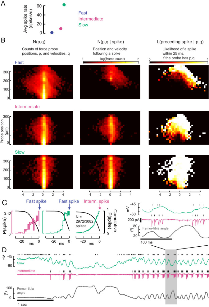
Figure 5u2014figure supplement 1.
Testing the recruitment hierarchy of motor neurons, in paired recordings and as a function of force probe position and velocity.
( A )u00a0The effective spike rate of fast, intermediate and slow motor neurons, over the course of all trials with spontaneous leg movements. Instantaneous spike rates could be much higher. ( B ) Fro...
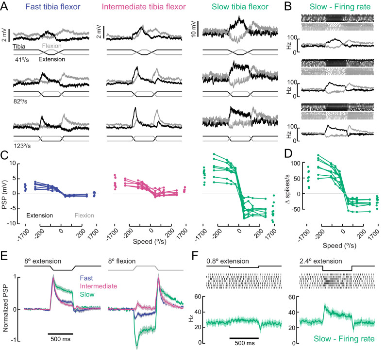
Figure 6.
A gradient of proprioceptive feedback to motor neurons controlling tibia flexion.
( A )u00a0Whole-cell recordings of fast, intermediate, and slow motor neurons in response to flexion (black) and extension (gray) of the tibia. Each trace shows the average membrane potential of a sin...
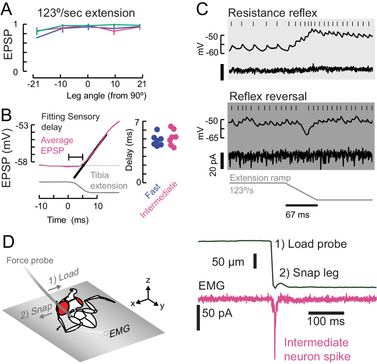
Figure 6u2014figure supplement 1.
Properties of sensory feedback to motor neurons.
( A )u00a0The EPSP evoked by fast ramping extension stimuli did not significantly depend on leg angle. ( B ) We measured the onset of the sensory evoked EPSP (magenta, intermediate neuron) in the moto...
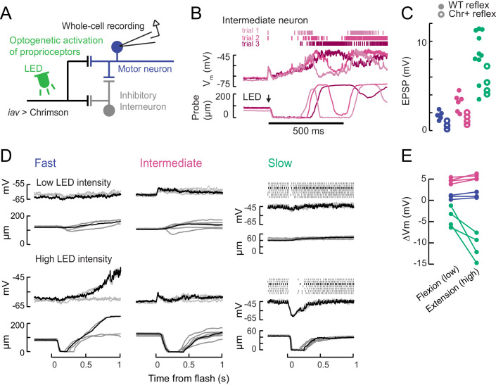
Figure 6u2014figure supplement 2.
Optogenetic activation of proprioceptive sensorimotor circuits.
( A )u00a0Optogenetic activation of proprioceptive feedback to tibia motor neurons. The axons of femoral chordotonal neurons, labeled by iav-LexA, were stimulated with Chrimson activation during whole...
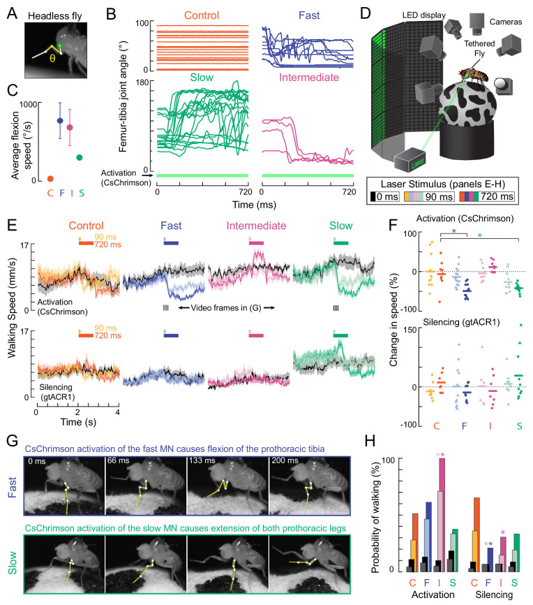
Figure 7.
Optogenetic perturbation of motor neurons in behaving flies.
( A )u00a0Example frame illustrating behavioral effects of optogenetically activating leg motor neurons in headless flies. A green laser (530 nm) is focused at the coxa-body joint of the flyu2019s lef...
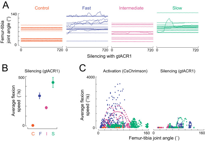
Figure 7u2014figure supplement 1.
Effects of tibia motor neuron silencing and activation on leg kinematics.
( A )u00a0Femur-tibia joint angles during silencing ( Gal4u00a0>gtACR1 ) of the three motor neuron types and a control empty Gal4 driver, in headless, suspended flies. ( B ) Average (u00b1u00a0sem) fl...
Video 3.
Optogenetic activation of motor neurons in headless flies.
The video shows the movements of the flies left front tibia caused by optogenetic activation of the fast, intermediate and slow neurons and a control line ( BDP-Gal4 ). The video shows 1) the tibia fl...
Video 4.
Optogenetic silencing in all motor neurons controlling the front leg.
Motor neurons labelled by OK371-Gal4 expressed gtACR1. The video shows the behavior of different flies on different trials while 1) flies were walking during a 90 ms laser stimulus; 2) flies were stat...
Video 5.
Optogenetic activation and silencing of fast motor neurons in behaving flies.
The video shows the behavior of different flies on different trials while 1) flies were walking and the fast neuron expressed CsChrimson; 2) flies were stationary, and the fast neuron expressed CsChri...
Video 6.
Optogenetic activation and silencing of intermediate motor neurons in behaving flies.
The video shows the behavior of different flies on different trials while 1) flies were walking and the intermediate neuron expressed CsChrimson; 2) flies were stationary, and the intermediate neuron ...
Video 7.
Optogenetic activation and silencing of slow motor neurons in behaving flies.
The video shows the behavior of different flies on different trials while 1) flies were walking and the slow neuron expressed CsChrimson; 2) flies were stationary, and the slow neuron expressed CsChri...
Video 8.
Optogenetic stimulation of a control line (BDP-Gal4).
The video shows the behavior of different control flies on different trials while 1) UAS-CsChrimson flies were walking; 2) UAS-CsChrimson flies were stationary; 3) UAS- gtACR1 flies were walking; 4) U...
Figure images are served from the NIH/NLM PubMed Central Open Access Subset or Europe PMC; copyright remains with the publishers and authors.
💬 Discussion
0 commentsNo comments yet. Be the first to start a discussion!
Leave a Comment