Abstract
Thylakoid membranes scaffold an assortment of large protein complexes that work together to harness the energy of light. It has been a longstanding challenge to visualize how the intricate thylakoid network organizes these protein complexes to finely tune the photosynthetic reactions. Previously, we used in situ cryo-electron tomography to reveal the native architecture of thylakoid membranes (Engel et al., 2015). Here, we leverage technical advances to resolve the individual protein complexes within these membranes. Combined with a new method to visualize membrane surface topology, we map the molecular landscapes of thylakoid membranes inside green algae cells. Our tomograms provide insights into the molecular forces that drive thylakoid stacking and reveal that photosystems I and II are strictly segregated at the borders between appressed and non-appressed membrane domains. This new approach to charting thylakoid topology lays the foundation for dissecting photosynthetic regulation at the level of single protein complexes within the cell.
🔬 Techniques
🧬 Organisms
✨ Fluorophores
🧪 Sample Preparation
🏭 Microscope Brands
💻 Software Details
💻 Code & Software
A tool for creating and analyzing panoramic views of biological membranes in electron tomograms.
A tool for creating and analyzing panoramic views of biological membranes in electron tomograms.
💾 Data Repositories
🏛️ Research Organizations (ROR)
Affiliated research institutions:
📋 Methods
Cell culture
We used the Chlamydomonas reinhardtii strains mat3-4 (CC-3994) ( Umen, 2001 ) and wild-type CC-125, provided by the Chlamydomonas Resource Center, University of Minnesota, MN. The mat3-4 strain has smaller cells that vitrify better by plunge freezing. Comparative 77K fluorescence measurements showed that mat3-4 and wild-type cells had similar spectra under the conditions that the cells were grown and frozen onto EM grids ( Figure 1—figure supplement 2 ). Thus, our description of the arrangement of photosynthetic complexes within mat3-4 thylakoids is likely comparable to wild-type thylakoids. For cryo-ET, mat3-4 cells were grown to mid-log phase (1000–2000 cells/μL) in Tris-acetate-phosphate (TAP) medium under constant light conditions (~90 µmol photons m −2 s −1 ) and bubbling with normal air. For 77K measurements, both mat3-4 and wild-type strains were grown under these same conditions, and measurements were made both immediately and after allowing cultures to sit in low light for 30 min.
77K measurements
Fresh colonies of CC-125 and CC-3944 were picked from agar plates and suspended in sterile air-bubbled flasks containing 50 mL TAP medium. The cultures were grown at room temperature under 90 µmol photons m −2 s −1 light until reaching 1,000 cells/μL. Samples containing 15 mL culture suspension were transferred into duplicate 15 mL Falcon tubes. From one of these tubes, five 1 mL aliquots were transferred to Eppendorf tubes and frozen immediately in liquid nitrogen. The second Falcon tube was kept under dim light of ~10 μmol photons m −2 s −1 for 30 min, with gentle mixing by inversion, and five 1 mL samples were then frozen as above. Fluorescence emission spectra were acquired as previously described ( Kanazawa et al., 2014 ) under liquid nitrogen, using a custom-made apparatus. Excitation was from a 440 nm diode laser, the output of which was sent through one branch of a bifurcated optical fiber (diameter of 1 mm) to the sample. The emission light was collected through the second fiber and measured with a spectrometer (Ocean Optics HR200 + ER). The average 77K profile for each condition was composed of three independent biological replicates, each with five technical replicates (15 measurements total per condition). Vitrification and Cryo-FIB milling Using a Vitrobot Mark 4 (FEI, Thermo Fisher Scientific), 4 µL of mat3-4 cell culture was blotted onto R2/1 carbon-coated 200-mesh copper EM grids (Quantifoil Micro Tools) and plunge frozen in a liquid ethane/propane mixture. Grids were stored in liquid nitrogen until used for FIB milling. Cryo-FIB milling was performed following a previously reported procedure ( Schaffer et al., 2015 ; Schaffer et al., 2017 ), using a Quanta dual-beam FIB/SEM instrument (FEI, Thermo Fisher Scientific), equipped with a Quorum PP3010 preparation chamber. Grids were clipped into Autogrid support rings modified with a cut-out on one side (FEI, Thermo Fisher Scientific). In the preparation chamber, the frozen grids were sputtered with a fine metallic platinum layer to make the sample conductive. Once loaded onto the dual-beam microscope’s cryo-stage, the grids were coated with a thicker layer of organometallic platinum using a gas injection system to protect the sample surface. After coating, the cells were milled with a gallium ion beam to produce ~100 nm-thick lamellas ( Figure 1 = 60–90 nm, Figure 1—figure supplement 1A = 100–140 nm, Figure 1—figure supplement 1C = 60–80 nm, Figure 1—figure supplement 1E = 110–140 nm). During transfer out of the microscope, the finished lamellas were coated with another fine layer of metallic platinum to prevent detrimental charging effects during Volta phase plate cryo-ET imaging, as previously described ( Mahamid et al., 2016 ; Schaffer et al., 2017 ). Cryo-ET After FIB milling, grids were transferred into a 300 kV Titan Krios microscope (FEI, Thermo Fisher Scientific), equipped with a Volta phase plate ( Danev et al., 2014 ), a post-column energy filter (Quantum, Gatan), and a direct detector camera (K2 summit, Gatan). Prior to tilt-series acquisition, the phase plate was conditioned to about 0.5π phase shift ( Danev et al., 2017 ). Using SerialEM software ( Mastronarde, 2005 ), bidirectional tilt-series (separated at 0°) were acquired with 2° steps between −60° and +60°. Individual tilts were recorded in movie mode with 12 frames per second, at an object pixel size of 3.42 Å and a target defocus of −0.5 µm. The total accumulated dose for the tilt-series was kept below ~100 e-/Å 2 . Each tomogram was acquired from a separate cell and thus is both a biological and technical replicate.
Show full methods section
Cell culture
We used the Chlamydomonas reinhardtii strains mat3-4 (CC-3994) ( Umen, 2001 ) and wild-type CC-125, provided by the Chlamydomonas Resource Center, University of Minnesota, MN. The mat3-4 strain has smaller cells that vitrify better by plunge freezing. Comparative 77K fluorescence measurements showed that mat3-4 and wild-type cells had similar spectra under the conditions that the cells were grown and frozen onto EM grids ( Figure 1—figure supplement 2 ). Thus, our description of the arrangement of photosynthetic complexes within mat3-4 thylakoids is likely comparable to wild-type thylakoids. For cryo-ET, mat3-4 cells were grown to mid-log phase (1000–2000 cells/μL) in Tris-acetate-phosphate (TAP) medium under constant light conditions (~90 µmol photons m −2 s −1 ) and bubbling with normal air. For 77K measurements, both mat3-4 and wild-type strains were grown under these same conditions, and measurements were made both immediately and after allowing cultures to sit in low light for 30 min.
77K measurements
Fresh colonies of CC-125 and CC-3944 were picked from agar plates and suspended in sterile air-bubbled flasks containing 50 mL TAP medium. The cultures were grown at room temperature under 90 µmol photons m −2 s −1 light until reaching 1,000 cells/μL. Samples containing 15 mL culture suspension were transferred into duplicate 15 mL Falcon tubes. From one of these tubes, five 1 mL aliquots were transferred to Eppendorf tubes and frozen immediately in liquid nitrogen. The second Falcon tube was kept under dim light of ~10 μmol photons m −2 s −1 for 30 min, with gentle mixing by inversion, and five 1 mL samples were then frozen as above. Fluorescence emission spectra were acquired as previously described ( Kanazawa et al., 2014 ) under liquid nitrogen, using a custom-made apparatus. Excitation was from a 440 nm diode laser, the output of which was sent through one branch of a bifurcated optical fiber (diameter of 1 mm) to the sample. The emission light was collected through the second fiber and measured with a spectrometer (Ocean Optics HR200 + ER). The average 77K profile for each condition was composed of three independent biological replicates, each with five technical replicates (15 measurements total per condition). Vitrification and Cryo-FIB milling Using a Vitrobot Mark 4 (FEI, Thermo Fisher Scientific), 4 µL of mat3-4 cell culture was blotted onto R2/1 carbon-coated 200-mesh copper EM grids (Quantifoil Micro Tools) and plunge frozen in a liquid ethane/propane mixture. Grids were stored in liquid nitrogen until used for FIB milling. Cryo-FIB milling was performed following a previously reported procedure ( Schaffer et al., 2015 ; Schaffer et al., 2017 ), using a Quanta dual-beam FIB/SEM instrument (FEI, Thermo Fisher Scientific), equipped with a Quorum PP3010 preparation chamber. Grids were clipped into Autogrid support rings modified with a cut-out on one side (FEI, Thermo Fisher Scientific). In the preparation chamber, the frozen grids were sputtered with a fine metallic platinum layer to make the sample conductive. Once loaded onto the dual-beam microscope’s cryo-stage, the grids were coated with a thicker layer of organometallic platinum using a gas injection system to protect the sample surface. After coating, the cells were milled with a gallium ion beam to produce ~100 nm-thick lamellas ( Figure 1 = 60–90 nm, Figure 1—figure supplement 1A = 100–140 nm, Figure 1—figure supplement 1C = 60–80 nm, Figure 1—figure supplement 1E = 110–140 nm). During transfer out of the microscope, the finished lamellas were coated with another fine layer of metallic platinum to prevent detrimental charging effects during Volta phase plate cryo-ET imaging, as previously described ( Mahamid et al., 2016 ; Schaffer et al., 2017 ). Cryo-ET After FIB milling, grids were transferred into a 300 kV Titan Krios microscope (FEI, Thermo Fisher Scientific), equipped with a Volta phase plate ( Danev et al., 2014 ), a post-column energy filter (Quantum, Gatan), and a direct detector camera (K2 summit, Gatan). Prior to tilt-series acquisition, the phase plate was conditioned to about 0.5π phase shift ( Danev et al., 2017 ). Using SerialEM software ( Mastronarde, 2005 ), bidirectional tilt-series (separated at 0°) were acquired with 2° steps between −60° and +60°. Individual tilts were recorded in movie mode with 12 frames per second, at an object pixel size of 3.42 Å and a target defocus of −0.5 µm. The total accumulated dose for the tilt-series was kept below ~100 e-/Å 2 . Each tomogram was acquired from a separate cell and thus is both a biological and technical replicate.
Tomogram reconstruction
Frame alignment was performed with K2Align ( https://github.com/dtegunov/k2align ). Using IMOD software ( Kremer et al., 1996 ), tilt-series were aligned with patch tracking, and bin4 reconstructions (13.68 Å pixel size) were created by weighted back projection. Of the 13 Volta phase plate tomograms acquired, four tomograms ( Figure 1 , Figure 1—figure supplement 1 ) were selected for analysis of photosynthetic complexes based on good IMOD tilt-series alignment scores and visual confirmation of well-resolved complexes at the thylakoid membranes.
Membrane segmentation
Segmentation of chloroplast membranes was performed in Amira software (FEI, Thermo Fisher Scientific), aided by automated membrane detection from the TomoSegMemTV package ( Martinez-Sanchez et al., 2014 ). Bin4 tomograms were processed with TomoSegMemTV to generate correlation volumes with high pixel intensity corresponding to membrane positions. The original bin4 tomograms and correlation volumes were imported into Amira, and the correlation volumes were segmented by 3D threshold-based selection, producing one-voxel-wide segmentations at the centers of the membranes. Using the 3D lasso selection tool, these segmentations were subdivided into appressed and non-appressed membrane regions ( Figure 1B , Figure 1—figure supplement 1B,D and F ). To generate membranograms visualizing complexes directly protruding from the membrane surface (PSII, PSI, cyt b 6 f ), the segmentations were grown by two voxels in all directions to produce a five-voxel-wide segmentation with a surface that matched the surface of the membrane. To generate membranograms visualizing complexes ~10 nm above the membrane surface (ATP synthase, membrane-bound ribosomes), segmentations were grown by 10 voxels in all directions. To produce smooth 3D surfaces, the segmented voxels were transformed into a polygonal mesh with the ‘generate surface’ command, decimated to 10% triangle density with the ‘remesh surface’ command, and smoothed with the ‘smooth surface’ command (50 iterations, 0.4 lambda). These surfaces were exported in the OBJ 3D model format.
Membranograms and particle picking
Bin4 tomograms and corresponding membrane segmentations (OBJ models) were loaded into Membranorama software ( https://github.com/dtegunov/membranorama ; copy archived at https://github.com/elifesciences-publications/membranorama ). This software projects tomographic density onto the surface of a 3D membrane segmentation to create a membranogram. Segmentations that had been grown by two voxels in Amira had surfaces that intersected densities protruding directly from the membrane surface (PSII, PSI, cyt b 6 f ). Segmentations that had been grown by 10 voxels in Amira had surfaces that intersected densities that were ~10 nm above the membrane surface (ATP synthase, membrane-bound ribosomes). Importantly, the Membranorama software can dynamically grow and shrink 3D membrane segmentations in real time, enabling the user to interactively track how densities appear at different distances from the membrane surface (see Video 2 ). The software also allows to-scale 3D models of each molecular complex (PDB: 6IJJ for PSI, 6KAD for PSII, 1Q90 for cyt b 6 f , 6FKF for ATP synthase, 5MMM for ribosome) ( Stroebel et al., 2003 ; Bieri et al., 2017 ; Hahn et al., 2018 ; Sheng et al., 2019 ; Su et al., 2019 ) to be mapped onto the membrane and compared to the tomographic densities. This is accomplished interactively by clicking the surface of the 3D membrane segmentation and using the mouse wheel to rotate each particle in the plane of the membrane. Using these features, we manually assigned membrane-associated densities to different classes of macromolecular complexes based on their positions relative to the membrane and their characteristic structural features ( Figure 2—figure supplement 1 ). For the luminal side of the membrane, we exclusively used segmentations that had been grown by two voxels. PSII was assigned to large dimeric densities projecting ~4 nm from the membrane surface, and cyt b 6 f was assigned to small dimeric densities projecting ~3 nm from the surface. For the stromal side of the membrane, we started with segmentations that had been grown by 10 voxels, assigning large round densities with ~25 nm diameters to ribosomes and smaller round densities with ~10 nm diameters to the F 1 subunit of ATP synthase. The stator of ATP synthase was often observed as a small density adjacent to the larger F 1 density (see Figure 2—figure supplement 1B ). After assigning the positions of these two complexes, we next loaded the corresponding segmentation that had been grown by two voxels and assigned PSI to small round densities projecting ~3 nm from the surface that were not positioned directly under a ribosome or ATP synthase. This order of particle picking prevented misassignment of PSI to the stalk of ATP synthase or the translocon structures that attach ribosomes to thylakoid membranes. The clarity of membrane-associated densities varied between different membranes within the same tomogram, likely due to effects of the tomographic missing wedge on different membrane curvatures and orientations, as well as local differences in the quality of tilt-series alignment. Therefore, only larger complexes (ribosomes, ATP synthase, PSII) were assigned for membranes with lower-clarity densities. Of the 51 non-appressed membranes quantified in this study, all complexes were assigned in 28 membranes, all complexes except for cyt b 6 f were assigned in two membranes, only ATP synthase and ribosomes were assigned in four membranes, and only ribosomes were assigned in 17 membranes. All complexes were assigned in the 33 appressed membranes quantified in this study. Within appressed membranes, PSII and cyt b 6 f were assigned with high confidence. Within non-appressed membranes, ribosomes and ATP synthase were assigned with high confidence, whereas PSI and cyt b 6 f were assigned with lower confidence (denoted by an asterisk in Table 1 ).
Subtomogram averaging
We used subtomogram averaging as a structural confirmation of the membranogram-picked positions for PSII and ATP synthase ( Figure 2—figure supplement 2 ). Manually assigned positions and orientations were exported from Membranorama and used as starting parameters for real space subtomogram alignment in PyTom software ( Hrabe et al., 2012 ). No classification was performed, and all membranogram-picked subvolumes were included in the averages (396 PSII particles, 639 ATP synthase particles).
Analysis of protein complex organization
Nearest-neighbor distances within the plane of a membrane To measure nearest-neighbor distances between molecular complexes within the thylakoids ( Figure 2—figure supplement 4 ), segmentations of essentially flat membrane regions were exported from Amira (FEI, Thermo Fisher Scientific) as MRC volumes. Coordinates of the particles (PSII, cyt b 6 f , ATP synthase, ribosomes) assigned on each membrane region were exported from Membranorama software. Each membrane region was projected with its corresponding particles onto a flat plane to generate a 2D surface. Nearest-neighbor distances between the particles were then measured using Matlab scripts calculating the shortest path between objects. Clustered poly-ribosomes exclude large regions of the stromal surface (see Figure 2C–D , Figure 2—figure supplement 3 ), which can cause misleading nearest-neighbor measurements for ATP synthase. To avoid this, the membranes were cropped to exclude regions containing poly-ribosome clusters before measuring ATP synthase distances. Overlap between adjacent membranes using EM densities To calculate overlap between EM densities from two adjacent membranes ( Figure 4F ), 11 membrane pairs separated by the stromal gap and six membrane pairs separated by the thylakoid lumen were segmented in Amira and imported into Membranorama software. Using the tools in Membranorama, surfaces from each membrane were selected and overlaid along a vector orthogonal to both membrane surfaces, ensuring a geometrically accurate superposition of the membrane densities. Images of the overlaid membranograms were then analyzed in Fiji software ( Schindelin et al., 2012 ) as described in Figure 4—figure supplement 1 . Thresholding and cropping the membranograms were necessary to decrease noise and avoid edge effects, respectively.
Overlap between adjacent membranes using membrane models
LHCII light-harvesting antennas are poorly visualized by cryo-ET because they are almost entirely embedded within the thylakoid membrane. Nevertheless, we incorporated hypothetical PSII-associated LHCII complexes into our analysis by using the PSII core positions and orientations visualized in membranograms to generate membrane models containing C 2 S 2 M 2 L 2 -type PSII-LHCII supercomplexes. First, 3D segmentations of appressed membrane regions were exported from Amira (FEI, Thermo Fisher Scientific). In the Membranorama software, we manually aligned a correctly scaled 3D model of the C 2 S 2 M 2 L 2 -type PSII-LHCII supercomplex (PDB: 6KAD) ( Sheng et al., 2019 ) with the EM densities observed for each PSII core particle. Coordinates and orientations of all the particles were exported from Membranorama. Using Matlab scripts, the PSII-LHCII supercomplex structure was filtered to 25 Å resolution and then mapped at the assigned positions and orientations into the 3D volume of the membrane segmentation, generating a 3D model of a one-voxel-thick membrane with embedded PSII-LHCII supercomplexes. To compare these experimentally determined models with simulated models containing randomly distributed supercomplexes, the same number of PSII-LHCII supercomplexes were placed one-by-one at random positions in the membrane (randomly selected voxels of the one-voxel-thick 3D membrane segmentation) and each time rotated by a random in-plane angle before placing the next supercomplex particle. Whenever a newly placed particle overlapped with a preexisting particle, rotation of the new particle was first attempted to avoid overlap, and if this failed, the particle was moved to a new random position (see Figure 4—figure supplement 2 for a 2D schematic representation of this 3D procedure). 100 random models were generated for each appressed membrane region. To measure the relative membrane area covered by the placed supercomplex structures ( Figure 4E ), the one-voxel-thick membrane segmentation was masked where it was intersected by the 3D structure volumes (PSII core alone, or PSII-LHCII supercomplexes of increasing size: C 2 S 2 -type, C 2 S 2 M 2 -type, and C 2 S 2 M 2 L 2 -type). This masked ‘occupied area’ was then divided by the total number of voxels in the membrane segmentation to yield a percentage. To calculate the overlap of ‘occupied area’ between adjacent membranes ( Figure 4F ), the C 2 S 2 M 2 L 2 -type supercomplex structure was subdivided into separate PSII (C 2 ) and LHCII (S 2 M 2 L 2 ) regions using Chimera software ( Goddard et al., 2007 ). Next, volumes of the complexes in one membrane were extended along a vector orthogonal to both membrane surfaces until they also intersected the adjacent membrane. These extended complex densities were then used to mask ‘occupied area’ on both membranes. Similar to the overlap calculation for EM density (detailed in Figure 4—figure supplement 1 ), the percent of overlap was calculated as the number of membrane voxels that were masked by complexes from both membranes (equivalent to white in Figure 4—figure supplement 1 ) divided by the sum of all masked voxels on the membrane (equivalent to white + green + magenta in Figure 4—figure supplement 1 ). ‘White’ overlap voxels masked by complexes from both membranes were only counted once in this calculation. The schematic models in Figure 4C–D provide a 2D representation of this 3D analysis.
Additional files Transparent reporting form
📊 Figures
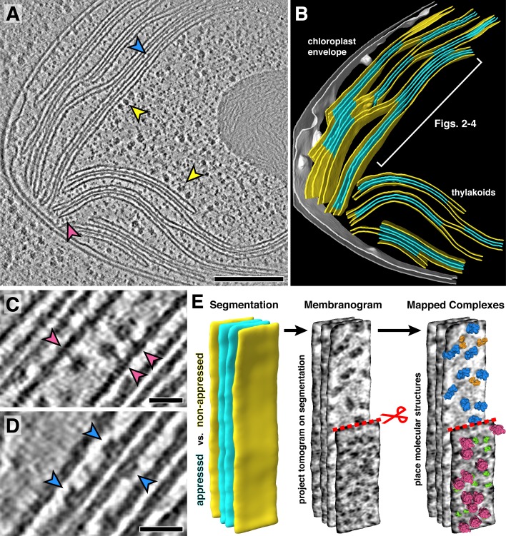
Figure 1.
In situ cryo-electron tomography reveals the native molecular architecture of thylakoid membranes.
( A ) Slice through a tomogram of the chloroplast within an intact Chlamydomonas cell. Arrowheads point to membrane-bound ribosomes (yellow), ATP synthase (magenta), and PSII (blue). ( B ) Correspondi...
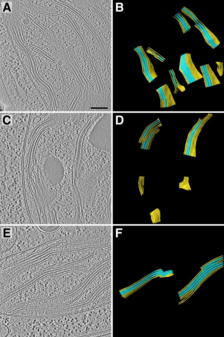
Figure 1u2014figure supplement 1.
Tomogram overviews.
Overviews of the three tomograms that were analyzed in addition to the tomogram shown in Figure 1 . ( A,u00a0C,u00a0E )u00a0Two-dimensional slices through the tomographic volumes. ( B,u00a0D,u00a0F )u...
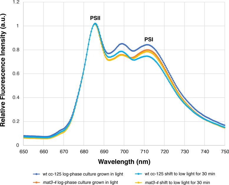
Figure 1u2014figure supplement 2.
The mat3-4 strain has a similar 77K fluorescence spectrum profile to wild-type cells.
Measurements were made from log-phase cultures grown under the same conditions that were used for cryo-ET (illuminated withu00a0~90 u00b5mol photons m u22122 s u22121 , bubbling with normal atmosphere...
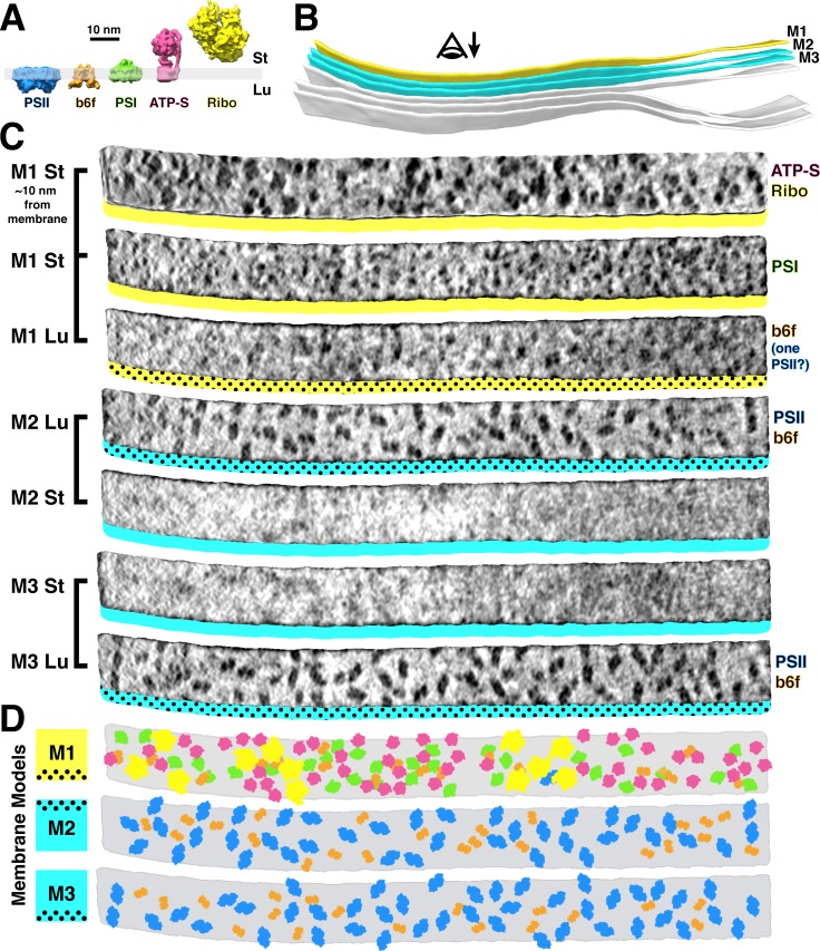
Figure 2.
Mapping photosynthetic complexes within appressed and non-appressed thylakoid membranes.
( A ) Schematic of how each molecular complex extends from the membrane into the stroma (St) and thylakoid lumen (Lu). Into the lumen, large dimeric densities extendu00a0~4 nm from PSII and small dime...
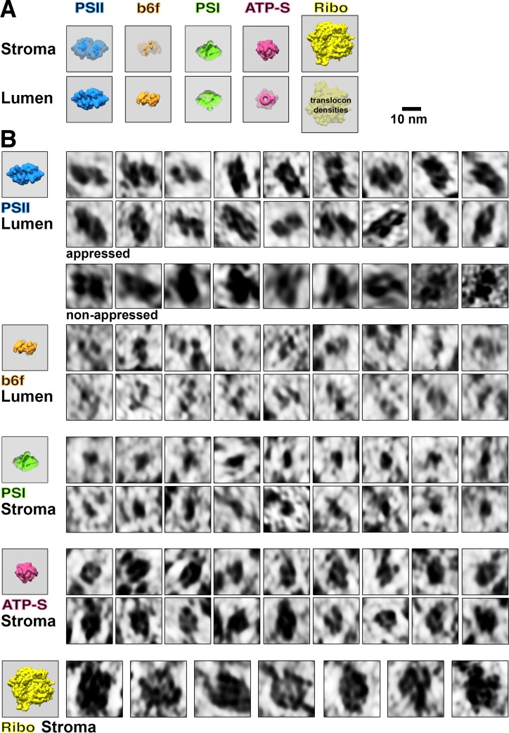
Figure 2u2014figure supplement 1.
Membranogram particle gallery.
( A ) Models of how each molecular complex appears when looking at the stromal and luminal surfaces of a thylakoid membrane (grey). Protruding densities are brightly colored, whereas densities located...
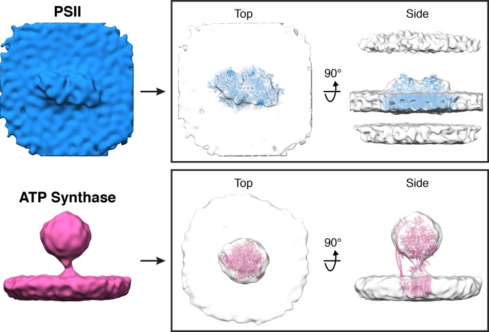
Figure 2u2014figure supplement 2.
Subtomogram averages of PSII and ATP synthase generated from particle positions assigned by membranograms.
In the boxes on the right, the averages are fitted with molecular structures determined by single particle cryo-EM (PDB: 6KAD, 6FKF) ( Hahn et al., 2018 ; Sheng et al., 2019 ). The subtomogram alignme...
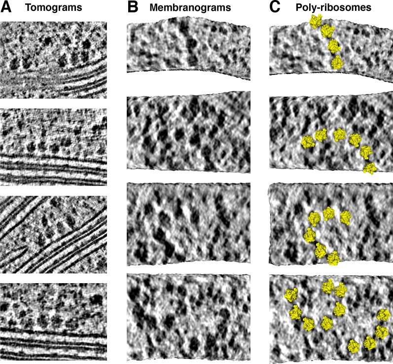
Figure 2u2014figure supplement 3.
Thylakoid-bound poly-ribosome chains.
( A ) Poly-ribosomes at thylakoid membranes, visualized in two-dimensional tomographic slices. ( B-C ) Poly-ribosome chains, ranging in length from 4 to 7 ribosomes, visualized in membranograms render...
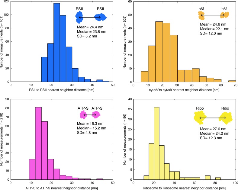
Figure 2u2014figure supplement 4.
Distributions of nearest-neighbor distances for PSII, cyt b 6 f , ATP synthase, and membrane-associated ribosomes.
Distances were measured between the center positions of nearest-neighbor complexes within the plane of the membrane. Mean, median, and standard deviation of the mean (SD) are noted in the plots. The P...
Video 1.
In situ cryo-electron tomography reveals native thylakoid architecture with molecular clarity.
Sequential slices back and forth in Z through the tomographic volume shown in Figure 1A . The yellow boxed region, focusing on the thylakoids shown in Figures 2 u2013 4 , is then enlarged and displaye...
Video 2.
Mapping molecular complexes into thylakoid architecture with membranograms.
Tomographic densities are projected onto the surface of a 3D membrane segmentation to produce a membranogram. The segmentation can be interactively grown and shrunk to visualize densities at different...
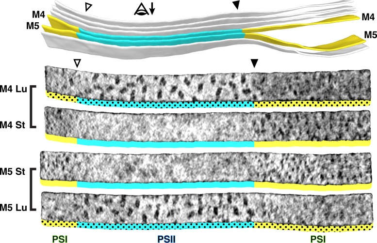
Figure 3.
Strict segregation of PSII and PSI at transitions between appressed and non-appressed regions.
Above: Three segmented thylakoids from the region indicated in Figure 1B . Membranes 4u20135 (M4 and M5, yellow: non-appressed, blue: appressed) are examined by membranograms. The eye symbol with arro...
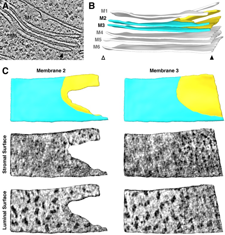
Figure 3u2014figure supplement 1.
Additional example of the strict lateral heterogeneity between PSI and PSII at the transition between appressed and non-appressed membrane domains.
( A ) Slice through a tomogram showing a stack of three thylakoids that splits into a stack of two thylakoids and a single thylakoid. ( B ) Segmentation of the thylakoid membranes in this stack. Arrow...
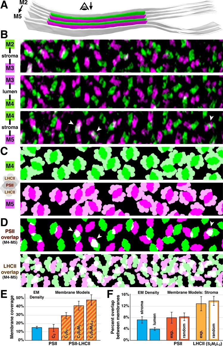
Figure 4.
Native thylakoids can accommodate PSII-LHCII supercomplexes, which are randomly distributed across the stromal gap.
( A ) Three segmented thylakoids from the region indicated in Figure 1B . Membranes 2u20135 (M2 to M5, alternating green and magenta) are examined by membranograms. The eye symbol with arrow indicates...
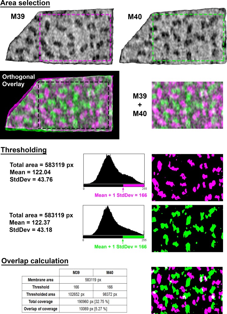
Figure 4u2014figure supplement 1.
Calculations of membrane coverage and intermembrane overlap from EM density.
Area selection: To select overlapping areas of two adjacent membranes (M39 and M40 in this example; magenta and green, respectively), the two membranograms are overlaid along a vector orthogonal to bo...
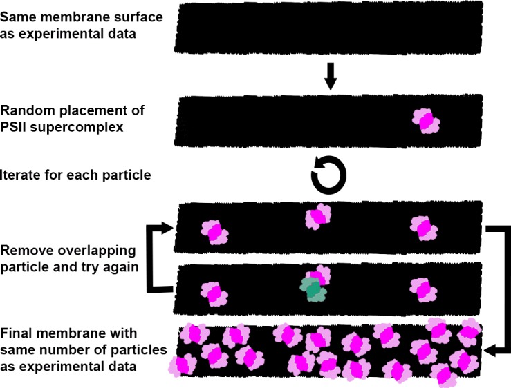
Figure 4u2014figure supplement 2.
Generation of random membrane models.
Schematic representation of the workflow for generating membranes with randomlyu00a0distributed C 2 S 2 M 2 L 2 -type PSII-LHCII supercomplexes, used for the analysis of intermembrane PSII and LHCII o...
Figure images are served from the NIH/NLM PubMed Central Open Access Subset or Europe PMC; copyright remains with the publishers and authors.
💬 Discussion
0 commentsNo comments yet. Be the first to start a discussion!
Leave a Comment