Abstract
Recent whole-brain mapping projects are collecting large-scale three-dimensional images using modalities such as serial two-photon tomography, fluorescence micro-optical sectioning tomography, light-sheet fluorescence microscopy, volumetric imaging with synchronous on-the-fly scan and readout or magnetic resonance imaging. Registration of these multi-dimensional whole-brain images onto a standard atlas is essential for characterizing neuron types and constructing brain wiring diagrams. However, cross-modal image registration is challenging due to intrinsic variations of brain anatomy and artifacts resulting from different sample preparation methods and imaging modalities. We introduce a cross-modal registration method, mBrainAligner, which uses coherent landmark mapping and deep neural networks to align whole mouse brain images to the standard Allen Common Coordinate Framework atlas. We build a brain atlas for the fluorescence micro-optical sectioning tomography modality to facilitate single-cell mapping, and used our method to generate a whole-brain map of three-dimensional single-neuron morphology and neuron cell types.
🔬 Techniques
🔭 Microscopes
💻 Software
✨ Fluorophores
🧪 Sample Preparation
🏭 Microscope Brands
🧪 Reagent Suppliers
🔴 Lasers
🔎 Objectives
🎨 Filters
💻 Software Details
📋 Protocols
💾 Data Repositories
🏛️ Research Organizations (ROR)
Affiliated research institutions:
📋 Methods
Microscope design
We constructed a microscope for fast volumetric STP tomography. The mouse brain, approximately 0.5 cm 3 in volume, requires 5 × 10 12 voxels for a full representation at a voxel size of 0.1 µm 3 . Acquiring this volume of data with conventional galvanometric scanning at a rate of 1 megavoxel/s would require about 4 months. We have developed a custom resonant scanning system capable of sustaining 16 megavoxels/s for up to 4 channels (128 MB/s data rate) to reduce imaging time to approximately 1 week per sample. The scan system is composed of a resonant scanning mirror (CRS-8kHz, Cambridge Technology, Bedford, MA) and a 5-mm linear scanning mirror (6215H, Cambridge Technology) conjugated with a scan telescope comprised of two custom scan objectives (Special Optics, Wharton, NJ) to ensure flat scanning across the available scan field. To avoid thermally damaging the sample at the edge of the resonant mirror scan field, an adjustable slit was placed at a conjugate image plane in the excitation path to block laser light in the appropriate area. A Pockels Cell (302RM, Conoptics, Danbury, CT) was used to modulate laser power and provide fast shuttering between frames. In this study, all imaging was performed using a 40×/1.3 NA oil-immersion objective (Objective Plan-Apochromat 40×/1.3 DIC, Carl Zeiss, Oberkochen, Germany). The emitted light was passed through a primary dichroic (FF735-Di01-25×36, Semrock, Rochester, NY) onto photomultiplier tubes (H7422P-40, Hamamatsu Photonics, Hamamatsu, Japan) using a custom detection head (part of the Janelia MIMMS microscope design) ( Flickinger et al., 2010 ). Two spectral channels were collected. eGFP emission was further filtered through a secondary dichroic (FF01-750/SP-25, Semrock) and an emission filter (FF03-525/50-30-D, Semrock). A second channel (FF02-617/73-30-D, Semrock) was collected for identification of red-labeled nuclei and/or spectral disambiguation of eGFP and broad-spectrum autofluorescence.
Show full methods section
Microscope design
We constructed a microscope for fast volumetric STP tomography. The mouse brain, approximately 0.5 cm 3 in volume, requires 5 × 10 12 voxels for a full representation at a voxel size of 0.1 µm 3 . Acquiring this volume of data with conventional galvanometric scanning at a rate of 1 megavoxel/s would require about 4 months. We have developed a custom resonant scanning system capable of sustaining 16 megavoxels/s for up to 4 channels (128 MB/s data rate) to reduce imaging time to approximately 1 week per sample. The scan system is composed of a resonant scanning mirror (CRS-8kHz, Cambridge Technology, Bedford, MA) and a 5-mm linear scanning mirror (6215H, Cambridge Technology) conjugated with a scan telescope comprised of two custom scan objectives (Special Optics, Wharton, NJ) to ensure flat scanning across the available scan field. To avoid thermally damaging the sample at the edge of the resonant mirror scan field, an adjustable slit was placed at a conjugate image plane in the excitation path to block laser light in the appropriate area. A Pockels Cell (302RM, Conoptics, Danbury, CT) was used to modulate laser power and provide fast shuttering between frames. In this study, all imaging was performed using a 40×/1.3 NA oil-immersion objective (Objective Plan-Apochromat 40×/1.3 DIC, Carl Zeiss, Oberkochen, Germany). The emitted light was passed through a primary dichroic (FF735-Di01-25×36, Semrock, Rochester, NY) onto photomultiplier tubes (H7422P-40, Hamamatsu Photonics, Hamamatsu, Japan) using a custom detection head (part of the Janelia MIMMS microscope design) ( Flickinger et al., 2010 ). Two spectral channels were collected. eGFP emission was further filtered through a secondary dichroic (FF01-750/SP-25, Semrock) and an emission filter (FF03-525/50-30-D, Semrock). A second channel (FF02-617/73-30-D, Semrock) was collected for identification of red-labeled nuclei and/or spectral disambiguation of eGFP and broad-spectrum autofluorescence.
High-fidelity synchronization of the digitizer and scan system
(Pockels cell, galvanometric scanner, and objective positioner) with the resonant mirror scan period was accomplished by reflecting a probe laser (635 nm, S1FC635PM, ThorLabs, Newton, NJ) from the resonant mirror onto a photodiode (PDA100A, Thorlabs). The photodiode was positioned 1 m away at one edge of the arc swept out by the resonant mirror. The voltage pulse generated by the incident probe laser was converted into a square wave using a custom circuit. This circuit was designed so that the rise of the square wave corresponds with the peak of the pulse observed from the photodiode, and permits adjustment of the clock phase in 5 ns increments. Collected photons were converted to an analog photocurrent, which was then amplified and converted to an analog voltage using a custom transimpedance amplifier (impulse response FWHM=25 ns), and digitized using a 12-bit high-speed digitizer at 125 Msamples/second (ATS-9350, AlazarTech, Pointe-Claire, Canada). A voltage bias was applied at the amplifier to take advantage of the digitizer’s full range. The digitizer generated records 16k samples wide at a rate of 8 kHz (256 MB/s/channel). These lines were distorted due to the spatially non-linear motion of the resonant mirror. Because of this, they were resampled using a cosine lookup table in a manner that is photoefficient (discards no samples) and avoids aliasing. Resampling was implemented on a GPU (GTX 580, NVidia, Santa Clara, CA) in order to meet data throughput requirements. Scanning a large volume of tissue was achieved by serially scanning a collection of smaller 3D stacks (tiles). Each of these tiles overlapped adjacent neighbors along each dimension, permitting post hoc registration. To address each tile, the sample was translated in three dimensions using a high-precision mechanical stage system (XY: M-511.DD, Z: M-501-DG, Controller: C843; Physike Instrumente, Karlsruhe, Germany). Fast scanning in the Z-direction was achieved using a piezo-electric motor to axially translate the objective (P-725K.103 and E-665.CR, Physike Instrumente). The maximum depth of each tile - typically set to 250 μm—was limited by the working distance of the objective and the range of the objective piezo. Integrated tissue sectioning was implemented on a custom assembly built around the vibrating servo from a Leica 1200S (Leica Microsystems, Wetzlar, Germany). Vibration was driven using an 86 Hz sine wave generated from a function generator and custom amplifier with vibration amplitude of approximately 1 mm. Tissue samples were positioned and fed across a stationary vibrating blade using the stage system at a velocity of 0.1 mm/sec. In this way, tissue sections >25 µm could be reliably removed from the tissue block once they were imaged. Computer aided design drawings and bill of materials are available at github.com/TeravoxelTwoPhotonTomography . Microscope operation Fully automated microscope operation was controlled by custom software (available at github.com/TeravoxelTwoPhotonTomography ). This software incorporates several features that ensure reliable operation spanning days to weeks. First, to guarantee an overlapping volume is reimaged after sectioning, the acquisition software applies a surface-finding procedure and adjusts the focal plane to ensure that tiles begin at the tissue surface. In this procedure, the surface is identified by searching for the top of the tissue by imaging autofluorescence in a subset of tiles with a coarse Z spacing around the expected surface position. Second, algorithms monitor the data quality of the incoming video stream to detect, for example, a photodetector fault. Third, to ensure that high data rates can be sustained over long acquisition times with high fidelity, data are locally cached on a solid-state hard drive (840 pro; Samsung) and asynchronously transferred to a highly-redundant network file system. Fourth, in the event of a fault, operation is safely halted and may resume from the point at which the fault occurred. Volume imaging is completed in a fully automatic process. After the top plane of the sample is positioned under the objective, a region of interest is determined by probing tiles across a designated search area. A single autofluorescence image is acquired at the bottom of each tile and classified based on whether it intersects the sample with a preset intensity threshold. When a tile that intersects the sample is found, neighboring tiles are searched in such a way as to trace the perimeter of the tissue. Tiles inside the perimeter are marked for imaging without being explicitly probed for efficiency. Finally the region of interest is dilated by one tile to ensure that tiles only partially intersecting the tissue sample are also acquired. The search process is finished when all the tiles in the search area have been classified. The marked region of interest is then imaged by sequentially volume-scanning constituent tiles. After all the tiles within the marked region of interest are imaged, the vibratome is engaged and a programmed stage motion feeds the sample through the blade to remove the top layer of tissue. The sample is translated back under the objective such that the newly exposed tissue surface is aligned with the focal plane and the process is repeated until no further tiles are found to image. Data was acquired in the coronal plane with tile dimensions of 386 × 422 × 250 μm (1024 × 1536 × 251 pixels) and an average dwell time of 61 ns/pixel. eGFP imaging was performed using a tunable ultrafast laser (Chameleon Ultra II, Coherent, Santa Clara, CA) at 920 nm using high excitation intensity (350–400 mW at the objective back aperture).
Image processing and registration
Image registration was implemented using custom scripts in Matlab (The MathWorks, Natick, MA). For laterally adjacent tiles, no registration was required; translating tiles using recorded stage positions was sufficient. For vertically adjacent tile pairs that spanned a sectioning plane, a set of corresponding features was determined using the descriptor-based image registration plugin in Fiji ( Preibisch et al., 2009 ). Because of the large number of tile pairs (>15,000 per brain), this procedure was distributed across a high-performance computing cluster. Compute time was approximately 1 min per tile pair (RAM 128 GB; 16 Intel E5-2680 CPUs). A set of common features, such as punctate auto-fluorescent bodies (lipofuscin; Figure 3—figure supplement 1 ) ( Dowson and Harris, 1981 ; Terman and Brunk, 2004 ), restricted to the putative overlap volume was successfully determined in approximately 2/3 of all tile pairs. Many of the remaining tile pairs either included little or no tissue (e.g. around the perimeter of the sample), or they were from relatively featureless areas within the tissue sample (e.g. ventricles and some white matter tracts). Next, point correspondences were aggregated across each tissue section and translated into the coordinate space defined by the stage system. From these point correspondences, a 3D displacement field was determined by fitting a cubic surface to the point cloud using the RegularizeData3d package for Matlab ( http://www.mathworks.com/matlabcentral/fileexchange/46223-regularizedata3d ). Although only axially-adjacent tile pairs were registered, tile pairs could be displaced relative to one another in all three Cartesian coordinates, necessitating the determination of deformation in three dimensions. This 3D displacement field was parameterized laterally for each (x,y) position across the section plane ( Figure 3b ). After the displacement fields between the current section and the sections above and below the current layer were determined, a 3D transform was computed to update the position of each tile within the full imaged volume. To solve for the transform, eight control points were determined for each tile at points offset slightly from the tile corners and located at the centroid of the overlap regions of neighboring tiles. Except in edge cases, there were seven overlapping tiles in the vicinity of each tile corner. These control points formed a regular grid across each section. Sampling the vector field at the centroid of these overlap regions is important for maintaining lateral continuity. We approximated the projection of these points from pixel space into the global coordinate space using a unique affine transform for each tile. Although useful for registration purposes, the presence of lipofuscin was sometimes undesirable during the tracing process even though these puncta were generally straightforward to disambiguate from labeled neurites. Due to the broad emission spectrum of these features, however, they could be computationally removed using standard linear spectral unmixing techniques. After this procedure, unmixed images - - computed from two-channel image tiles - contained only eGFP-labeled structures. Images in Figures 3 – 5 and Video 1 were unmixed according to U = G − kR , where U is the unmixed image, G is the green channel of the original image, and R is the red channel of the original image. k is an empirically-determined scale factor.
Image visualization and annotation
For the purposes of viewing and annotating datasets, all of the tiles in each dataset (input tiles) were resampled into a common coordinate space according to the individual affine transforms determined during the registration procedure. This produced a set of axis-aligned non-overlapping image stacks (output tiles) spanning the imaged volume. Resampling was achieved by back-projecting each voxel in each output tile to one or more input tiles where the nearest voxel was sampled. To avoid aliasing, input tiles were pre-filtered with a Gaussian kernel (sigma = 150 nm). In regions where two or more input tiles overlapped, the maximum intensity was used for the corresponding location in the output tile. The resampling task was implemented on a GPU, which ensured that execution time was dominated by the time required to read input data. Work was distributed output tile-wise over a GPU cluster (20 nodes with 7× GTX 580 1.5GB VRAM). Importantly, each node had parallel access to high-bandwidth network storage. Data were resampled to voxels 0.3 × 0.3 × 1 µm, and stored on disk along with hierarchically downsampled representations of the same volume for visualization at different spatial scales. In order to smoothly navigate and annotate neuronal structures across large volumes of rendered data, we used a custom plugin for the Janelia Workstation ( Murphy et al., 2014 ) that displays and predictively pre-caches multiresolution data using a scheme similar to that employed for large imaging datasets in electron microscopy ( Anderson et al., 2011 ; Cardona et al., 2012 ; Saalfeld et al., 2009 ). The neuronal structures depicted in this study were reconstructed by manually placing control points approximately every 5–10 µm and were stored using the SWC file format. Manual reconstruction of neurons required approximately 10–30 min/mm and speed depended upon labeling density, signal intensity, and annotator experience. Image compression To archive datasets, raw data was compressed using the H.264 format (libavcodec; parameters: crf 18, preset slow, tune film). Each color channel was compressed independently as a 16-bit grayscale volume. Compression of a full dataset was distributed, tile-wise, using a high-performance compute cluster. Compressed datasets were typically ~1 TB/channel in size.
Development of clearing protocol
DMSO has a high refractive index (1.479) and is used extensively in mounting medium formulations for fluorescence microscopy. To improve the clearing properties of DMSO, we investigated solutions of DMSO containing a sugar or sugar alcohol, based on the established tissue-clearing properties of these molecules. We examined the solubility of several compounds: sucrose, d -fructose, d -mannitol, d -sorbitol, xylitol, maltitol, and meso -erythritol. We found that d -sorbitol was highly soluble in DMSO up to 1 g d -sorbitol per 1 ml DMSO (44% w/w). Although the saturated solution of d -sorbitol in DMSO was an effective tissue-clearing agent, this organic environment irreversibly decreased the fluorescence of eGFP in tissue slices. We therefore measured the fluorescence of purified eGFP as a function of DMSO concentrations (in 10 mM HEPES, pH 7.3) with or without d -sorbitol ( Figure 2b ). Surprisingly, eGFP fluorescence increased modestly at low concentrations of DMSO followed by a severe decrease at 70% v/v DMSO without d -sorbitol and at 80% v/v DMSO in solutions that included d -sorbitol. We then screened ternary mixtures of DMSO/H 2 O/ d -sorbitol, to produce the clearing protocol described in Table 1 , which uses increasing amounts of d -sorbitol with a final concentration of 45% w/w d -sorbitol in a solvent made up of 60% v/v DMSO in 0.01 M phosphate buffer. Increasing the concentration of d -sorbitol to its solubility limit (63% w/w; Solution #6 in Table 1 ) further improved clearing, but evaporation and mechanical agitation initiated precipitation of d -sorbitol and/or gel formation during sectioning and imaging.
Tissue processing and clearing
Mice were deeply anesthetized with an overdose of isoflurane and transcardially perfused with PBS that included 20 U/ml heparin (H3393; Sigma-Aldrich, St. Louis, MO) followed by 4% paraformaldehyde in PBS. Brains were extracted immediately following perfusion and post-fixed for 4 hr at 4°C and washed 3× in 0.1 PBS for >1 hr each. Brains were immersed in CUBIC-1 ( Susaki et al., 2014 ) for 3–7 days to remove lipids and subsequently washed 3× in PBS for >1 hr each. Nuclei of samples were optionally counter-stained with 10 µM NuclearID-Red solution (ENZ-52406, Enzo Life Sciences, Farmingdale, NY), washed, embedded in gelatin (12% w/v in PB) and fixed in 4% paraformaldehyde for 12 hr. Cross-linking the tissue to the gelatin embedding medium enabled stable, high SNR imaging even when only a thin section of material remained. Embedded samples were subsequently cleared by immersion in solutions #1–5 ( Table 1 ) (1 day in each step). DMSO (472301) and d -sorbitol (85529) were obtained from Sigma-Aldrich. High-purity d -sorbitol was found to be necessary to ensure the absence of fluorescent contaminants. PB and PBS were used at 0.01 M and 0.1 M, respectively.
Viral labeling
High titer (> 10 12 GC/ml) AAV 2/1 Syn-iCre and AAV 2/1 CAG-Flex-eGFP were obtained from the Janelia Research Campus Molecular Biology Core. The Cre virus was diluted 1:45,000 in sterile water and combined at a 1:1 ratio with the eGFP virus for injections into the motor cortex of C57/BL6 mice (M/L +0.7; A/P +1.3; D/V −0.75, −0.5, −0.25 relative to bregma; 30 nl/depth). All experimental protocols were conducted according to the National Institutes of Health guidelines for animal research and were approved by the Institutional Animal Care and Use Committee at Howard Hughes Medical Institute Janelia Research Campus (Protocol #14–115).
Development of clearing protocol
DMSO has a high refractive index (1.479) and is used extensively in mounting medium formulations for fluorescence microscopy. To improve the clearing properties of DMSO, we investigated solutions of DMSO containing a sugar or sugar alcohol, based on the established tissue-clearing properties of these molecules. We examined the solubility of several compounds: sucrose, d -fructose, d -mannitol, d -sorbitol, xylitol, maltitol, and meso -erythritol. We found that d -sorbitol was highly soluble in DMSO up to 1 g d -sorbitol per 1 ml DMSO (44% w/w). Although the saturated solution of d -sorbitol in DMSO was an effective tissue-clearing agent, this organic environment irreversibly decreased the fluorescence of eGFP in tissue slices. We therefore measured the fluorescence of purified eGFP as a function of DMSO concentrations (in 10 mM HEPES, pH 7.3) with or without d -sorbitol ( Figure 2b ). Surprisingly, eGFP fluorescence increased modestly at low concentrations of DMSO followed by a severe decrease at 70% v/v DMSO without d -sorbitol and at 80% v/v DMSO in solutions that included d -sorbitol. We then screened ternary mixtures of DMSO/H 2 O/ d -sorbitol, to produce the clearing protocol described in Table 1 , which uses increasing amounts of d -sorbitol with a final concentration of 45% w/w d -sorbitol in a solvent made up of 60% v/v DMSO in 0.01 M phosphate buffer. Increasing the concentration of d -sorbitol to its solubility limit (63% w/w; Solution #6 in Table 1 ) further improved clearing, but evaporation and mechanical agitation initiated precipitation of d -sorbitol and/or gel formation during sectioning and imaging.
📊 Figures
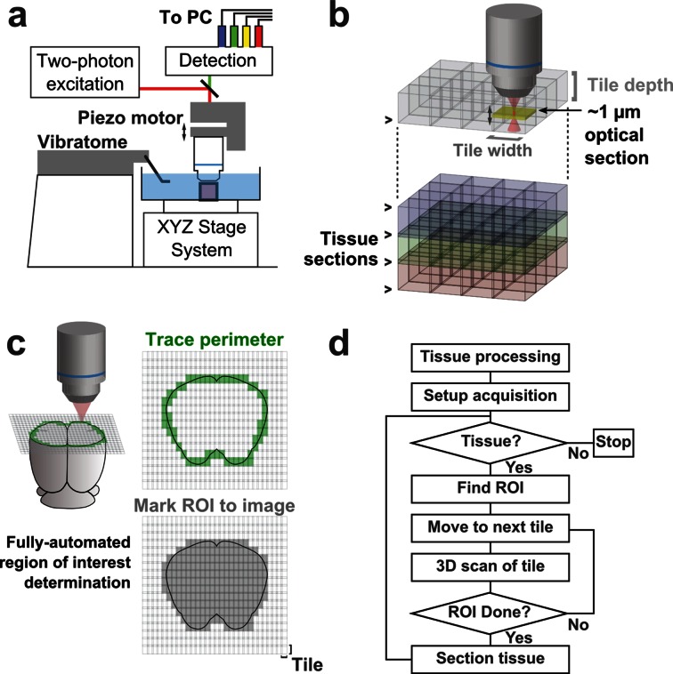
Figure 1.
Schematic of imaging system.
( a ) Schematic of apparatus for automated volumetric two-photon tomography. ( b ) To image large volumes of tissue, a collection of three-dimensional image stacks (tiles) covering the full volume of ...
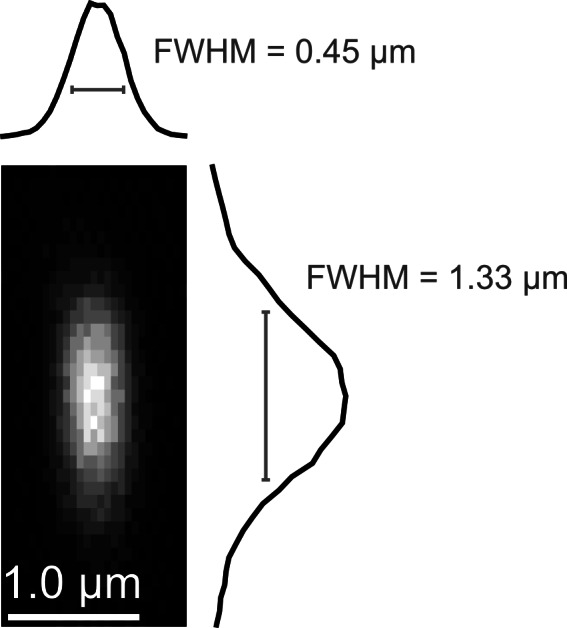
Figure 1u2014figure supplementu00a01.
Point spread function measurement.
( a ) Empirically-measured point spread function measured using 200-nm fluorescent polystyrene beads. DOI: http://dx.doi.org/10.7554/eLife.10566.004
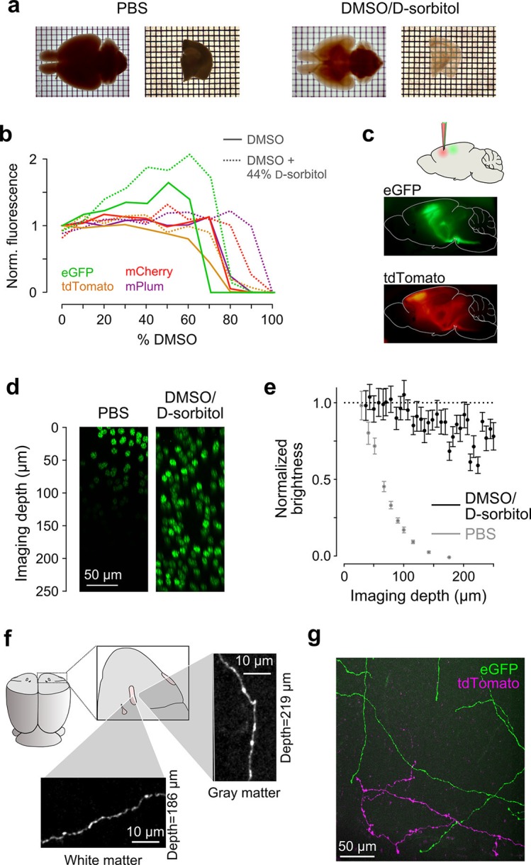
Figure 2.
Sample preparation and clearing.
( a ) Whole brains ( left ) and 1 mm-thick tissue sections ( right ) cleared using dimethyl sulfoxideu00a0(DMSO) and d -sorbitol. ( b ) Fluorescence of purified eGFP as a function of DMSO concentratio...
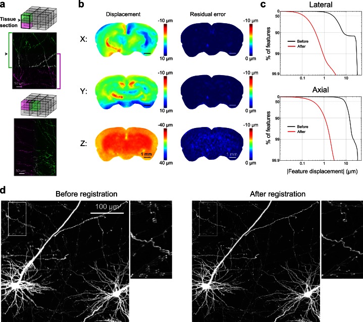
Figure 3.
Registration of image tiles.
( a ) Example registration of pairs of image tiles in the axial (left) and lateral (right) directions. ( b ) Initial displacement of automatically-identified features as a result of sectioning ( left ...
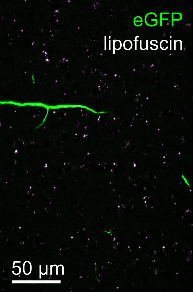
Figure 3u2014figure supplement 1.
Lipofuscin imaging.
Overlay of fluorescence captured in the green (500u2013550 nm) and orange (580u2013653 nm) spectral bands from a representative tile within the neocortex. Autofluorescent lipofuscin (white puncta) cou...
Video 1.
Movie illustrating 18 serially acquired image tiles that have been registered and resampled into a continuous image volume.
This volume (3u00a0u00d7u00a01u00a0u00d7u00a06 tiles) spans five adjacent tissue sections. Fine axons are resolvable and all fibers appear continuous. Images were spectrally unmixed to remove autofluo...
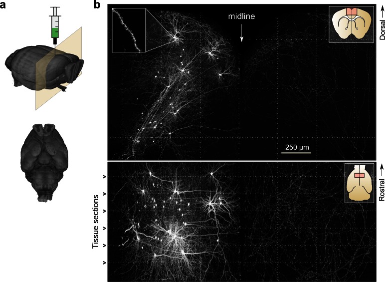
Figure 4.
Whole-brain imaging.
( a ) Three-dimensionalu00a0rendering of complete mouse brain dataset as viewed from an anterolateral ( left ) and ventral ( right ) perspective. ( b ) Maximumu00a0intensity projection through a large...
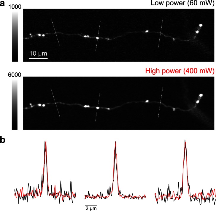
Figure 4u2014figure supplement 1.
High speed, high-power imaging.
( a ) Image of an axonal collateral with low ( top ) and high ( bottom ) excitation power. High-power imaging improves signal-to-noise without degrading resolution due to fluorophore saturation. ( b )...
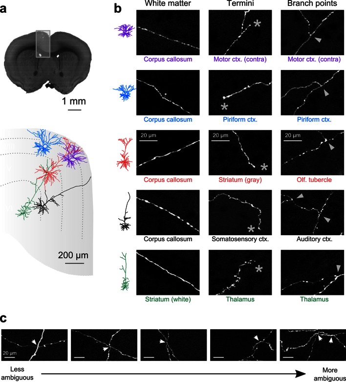
Figure 5.
Axon collaterals are labeled with high signal-to-noise across their entire length.
( a ) Top: Virtual coronal section through whole-brain dataset. Boxed area denotes region containing labeled somata and is expanded in schematic below. Bottom: Laminar distribution and dendritic morph...
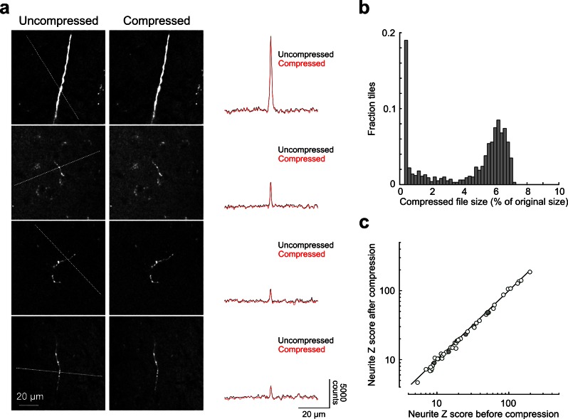
Figure 5u2014figure supplement 1.
Signal-to-noise of axonal imaging.
( a ) Representative images before ( left ) and after ( middle ) lossy H.264 compression. The intensity profile across each neurite (along paths denoted by dotted lines in images on left) is plotted t...
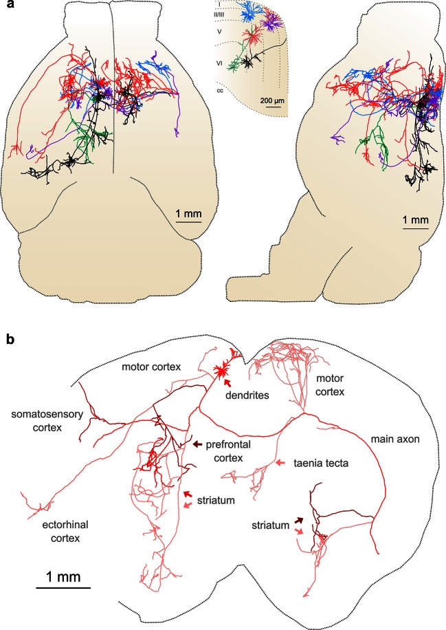
Figure 6.
Complete reconstruction of axonal morphology.
( a ) Complete reconstruction of the same five projection neurons depicted in Figure 4 (inset). Reconstructions are overlaid on a horizontal ( left ) and sagittal ( right ) outline of the imaged mouse...
Video 2.
Single axon traced to its terminus.
Depicted path represents the longest continuous axonal segment starting at the cell soma. The terminus is located in the anterior piriform cortex. White dot corresponds to the same location in both pa...
Video 3.
Three-dimensional rendering of reconstructed Layer II motor cortical neurons.
Displayed brain outline corresponds to the contours of the imaged brain. Color code is the same as in all figures. DOI: http://dx.doi.org/10.7554/eLife.10566.017
Video 4.
Three-dimensional rendering of reconstructed Layer V motor cortical neurons.
Displayed brain outline corresponds to the contours of the imaged brain. Color code is the same as in all figures. DOI: http://dx.doi.org/10.7554/eLife.10566.018
Video 5.
Three-dimensional rendering of reconstructed Layer VI motor cortical neuron.
Displayed brain outline corresponds to the contours of the imaged brain. Color code is the same as in all figures. DOI: http://dx.doi.org/10.7554/eLife.10566.019
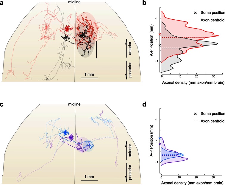
Figure 7.
Fine scale topology of contralateral cortical projections.
( a ) Horizontal view of the dendrites and axons of two layer V IT neurons (red and black). Axons projecting to locations other than the contralateral motor cortex are shown in lighter colors. ( b ) D...
Figure images are served from the NIH/NLM PubMed Central Open Access Subset or Europe PMC; copyright remains with the publishers and authors.
💬 Discussion
0 commentsNo comments yet. Be the first to start a discussion!
Leave a Comment