Abstract
Point-scanning imaging systems are among the most widely used tools for high-resolution cellular and tissue imaging, benefiting from arbitrarily defined pixel sizes. The resolution, speed, sample preservation and signal-to-noise ratio (SNR) of point-scanning systems are difficult to optimize simultaneously. We show these limitations can be mitigated via the use of deep learning-based supersampling of undersampled images acquired on a point-scanning system, which we term point-scanning super-resolution (PSSR) imaging. We designed a 'crappifier' that computationally degrades high SNR, high-pixel resolution ground truth images to simulate low SNR, low-resolution counterparts for training PSSR models that can restore real-world undersampled images. For high spatiotemporal resolution fluorescence time-lapse data, we developed a 'multi-frame' PSSR approach that uses information in adjacent frames to improve model predictions. PSSR facilitates point-scanning image acquisition with otherwise unattainable resolution, speed and sensitivity. All the training data, models and code for PSSR are publicly available at 3DEM.org.
🔬 Techniques
🔭 Microscopes
💻 Software
✨ Fluorophores
🧪 Sample Preparation
🔬 Cell Lines
🏭 Microscope Brands
🧪 Reagent Suppliers
📷 Detectors
🔎 Objectives
💻 Software Details
💻 Code & Software
💾 Data Repositories
🏛️ Research Organizations (ROR)
Affiliated research institutions:
📋 Methods
Semi-synthetic Training Image Generation
HR images were acquired using scanning electron or Airyscan confocal microscopes. Due to the variance of image properties (e.g. format, size, dynamic range and depth) in the acquired HR images, data cleaning is indispensable for generating training sets that can be easily accessed during training. In this article, we differentiate the concept of “data sources” and “data sets”, where data sources refer to uncleaned acquired high-resolution images, while data sets refer to images that are generated and preprocessed from data sources. HR data sets were obtained after preprocessing HR images from data sources, LR data sets were generated from HR data sets using a “crappifier” function. Preprocessing. Tiles of predefined sizes (e.g. 256 × 256 and 512 × 512 pixels) were randomly cropped from each frame in image stacks from HR data sources. “Refection padding” was used if the image size in the data sources is smaller than the predefined tile size. All tiles were saved as separate images in .tif format, which together formed a HR data set. Image Crappification. A “crappifier” was then used to synthetically degrade the HR data sets to LR images, with the goal of approximating the undesired and unavoidable pixel intensity variation in real-world low-resolution and low SNR images of the same field of view directly taken under an imaging system. These HR images together with their corrupted counterparts served as training pairs to facilitate “deCrappification”. The crappification function can be simple, but it materially improves both the quality and characteristics of PSSR outputs. Image sets were normalized from 0 to 1 before being 16x downsampled in pixel resolution (e.g. a 1000 × 1000 pixel image would be downsampled to 250 × 250 pixels). To mimic the image quality degradation caused by 16x undersampling on a real-world point-scanning imaging system, salt-and-pepper noise, and Gaussian additive noise with specified local variance were randomly injected into the high-resolution images. The degraded images were then rescaled to 8-bit for viewing with normal image analysis software. EM Crappifier Random Gaussian-distributed additive noise ( μ E M = 0 , σ E M = 3 ) was injected. The degraded images were then downsampled using spline interpolation of order 1. MitoTracker and Neuronal Mitochondria Crappifier The crappification of MitoTracker and neuronal mitochondria data followed a similar procedure. Salt-and-pepper noise was randomly injected in 0.5% of each image’s pixels replacing them with noise, which was followed by the injection of random Gaussian-distributed additive noise ( μ L S M = 0 , σ L S M = 5 ). The crappified images were then downsampled using spline interpolation of order 1. Data Augmentation. After crappified low-resolution images were generated, we used data augmentation techniques such as random cropping, dihedral affine function, rotation, random zoom to increase the variety and size of our training data 40 . Multi-frame Training Pairs. Unlike imaging data of fixed samples, where we use traditional one-to-one high- and low-resolution images as training pairs, for time-lapse movies, five consecutive frames ( H R i , i ∈ t - 2 , t + 2 ) from a HR Airyscan time-lapse movie were synthetically crappified to five LR images ( L R i , i ∈ t - 2 , t + 2 ), which together with the HR middle frame at time t ( H R t ) , form a five-to-one training “pair”. The design of five-to-one training “pairs” leverages the spatiotemporal continuity of dynamic biological behaviors. ( Fig. 4a ).
Show full methods section
Semi-synthetic Training Image Generation
HR images were acquired using scanning electron or Airyscan confocal microscopes. Due to the variance of image properties (e.g. format, size, dynamic range and depth) in the acquired HR images, data cleaning is indispensable for generating training sets that can be easily accessed during training. In this article, we differentiate the concept of “data sources” and “data sets”, where data sources refer to uncleaned acquired high-resolution images, while data sets refer to images that are generated and preprocessed from data sources. HR data sets were obtained after preprocessing HR images from data sources, LR data sets were generated from HR data sets using a “crappifier” function. Preprocessing. Tiles of predefined sizes (e.g. 256 × 256 and 512 × 512 pixels) were randomly cropped from each frame in image stacks from HR data sources. “Refection padding” was used if the image size in the data sources is smaller than the predefined tile size. All tiles were saved as separate images in .tif format, which together formed a HR data set. Image Crappification. A “crappifier” was then used to synthetically degrade the HR data sets to LR images, with the goal of approximating the undesired and unavoidable pixel intensity variation in real-world low-resolution and low SNR images of the same field of view directly taken under an imaging system. These HR images together with their corrupted counterparts served as training pairs to facilitate “deCrappification”. The crappification function can be simple, but it materially improves both the quality and characteristics of PSSR outputs. Image sets were normalized from 0 to 1 before being 16x downsampled in pixel resolution (e.g. a 1000 × 1000 pixel image would be downsampled to 250 × 250 pixels). To mimic the image quality degradation caused by 16x undersampling on a real-world point-scanning imaging system, salt-and-pepper noise, and Gaussian additive noise with specified local variance were randomly injected into the high-resolution images. The degraded images were then rescaled to 8-bit for viewing with normal image analysis software. EM Crappifier Random Gaussian-distributed additive noise ( μ E M = 0 , σ E M = 3 ) was injected. The degraded images were then downsampled using spline interpolation of order 1. MitoTracker and Neuronal Mitochondria Crappifier The crappification of MitoTracker and neuronal mitochondria data followed a similar procedure. Salt-and-pepper noise was randomly injected in 0.5% of each image’s pixels replacing them with noise, which was followed by the injection of random Gaussian-distributed additive noise ( μ L S M = 0 , σ L S M = 5 ). The crappified images were then downsampled using spline interpolation of order 1. Data Augmentation. After crappified low-resolution images were generated, we used data augmentation techniques such as random cropping, dihedral affine function, rotation, random zoom to increase the variety and size of our training data 40 . Multi-frame Training Pairs. Unlike imaging data of fixed samples, where we use traditional one-to-one high- and low-resolution images as training pairs, for time-lapse movies, five consecutive frames ( H R i , i ∈ t - 2 , t + 2 ) from a HR Airyscan time-lapse movie were synthetically crappified to five LR images ( L R i , i ∈ t - 2 , t + 2 ), which together with the HR middle frame at time t ( H R t ) , form a five-to-one training “pair”. The design of five-to-one training “pairs” leverages the spatiotemporal continuity of dynamic biological behaviors. ( Fig. 4a ).
Crappifier comparison
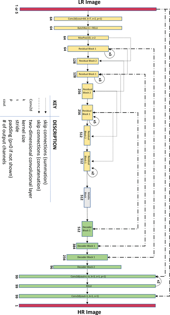
EM crappifier comparison. Four crappifiers including “No noise”, “Poisson”, “Gaussian” and “Additive Gaussian” were used to generate semi-synthetic training pairs from the same set of HR SEM images. The “No noise” crappifier simply downsampled HR image pixel sizes by a factor of 16x (4×4) without adding any noise, while the “Poisson”, “Gaussian” and “Additive Gaussian” crappifiers added random Poisson noise, random Gaussian noise ( μ E M = 0 , σ E M = 0.15 ) and random Gaussian-distributed additive noise ( μ E M = 0 , σ E M = 3 ) respectively, before applying pixel downsampling. “Additive Gaussian (~80x)” used the same crappifier as “Additive Gaussian”, but with ~80x more training data. We also compared the models described above with “Real-world”, a model trained with real-world pairs, whose HR images are the same as the HR images of the semi-synthetically generated training pairs, but whose LR images were manually acquired at the microscope. MitoTracker crappifier comparison. Five crappifiers including “No noise”, “Salt & Pepper”, “Gaussian”, “Additive Gaussian” and “Salt & Pepper + Additive Gaussian” were used to generate semi-synthetic training pairs from the same set of HR Airyscan MitoTracker time-lapse videos. The “No noise” crappifier downsampled HR image pixel sizes by a factor of 16x (4×4) without adding any noise, while the “Salt & Pepper”, “Gaussian”, “Additive Gaussian”, and “Salt & Pepper + Additive Gaussian” crappifiers added random Salt & Pepper noise (0.5%), random Gaussian noise ( μ L S M = 0 , σ L S M = 0.025 ), random Gaussian-distributed additive noise ( μ L S M = 0 , σ L S M = 5 ), and the combination of “Salt & Pepper” and “Additive Gaussian” respectively, before the bilinear downsampling. Neural Networks Single-frame Neural Network (PSSR-SF). A ResNet-based U-Net was used as our convolutional neural network for training 41 . Our U-Net is in the form of encoder-decoder with skip-connections, where the encoder gradually downsizes an input image, followed by the decoder upsampling the image back to its original size. For the EM data, we utilized ResNet pretrained on ImageNet as the encoder. For the design of the decoder, the traditional handcrafted bicubic upscaling filters are replaced with learnable sub-pixel convolutional layers 42 , which can be trained specifically for upsampling each feature map optimized in low-resolution parameter space. This upsampling layer design enables better performance and largely reduces computational complexity, but at the same time causes unignorable checkerboard artifacts due to the periodic time-variant property of multirate upsampling filters 43 . A blurring technique 44 and a weight initialization method known as “sub-pixel convolution initialized to convolution neural network resize (ICNR)” 45 designed for the sub-pixel convolution upsampling layers were implemented to remove checkerboard artifacts. In detail, the blurring approach introduces an interpolation kernel of the zero-order hold with the scaling factor after each upsampling layer, the output of which gives out a non-periodic steady-state value, which satisfies a critical condition ensuring a checkerboard artifact-free upsampling scheme 44 . Compared to random initialization, in addition to the benefit of removing checkerboard artifacts, ICNR also empowers the model with higher modeling power and higher accuracy 45 . A self-attention layer inspired by Zhang et al. 46 was added after each convolutional layer. Multi-frame Neural Network (PSSR-MF). A similar yet slightly modified U-Net was used for time-lapse movie training. The input layer was redesigned to take five frames simultaneously while the last layer still produced one frame as output. Training Details Loss Function. MSE loss was used as our loss function. Optimization Methods. Stochastic gradient descent with restarts (SGDR) 47 was implemented. Aside from the benefits we are able to get through classic stochastic gradient descent, SGDR resets the learning rate to its initial value at the beginning of each training epoch and allows it to decrease again following the shape of a cosine function, yielding lower loss with higher computational efficiency.
Cyclic Learning
Rate and Momentum. Instead of having a gradually decreasing learning rate as the training converges, we adopted cyclic learning rates 48 , cycling between upper bound and lower bound, which helps oscillate towards a higher learning rate, thus avoiding saddle points in the hyper-dimensional training loss space. In addition, we followed The One Cycle Policy 49 , which restricts the learning rate to only oscillate once between the upper and lower bounds. Specifically, the learning rate linearly increases from the lower bound to the upper bound as the momentum decreases from its upper bound to the lower bound linearly. In the second half of the cycle, the learning rate fits a cosine annealing decreasing from the upper bound to zero while the momentum increases from its lower bound to the upper bound following the same annealing. This training technique achieves superior regularization by preventing the network from overfitting during the middle of the learning process, as well as enables super-convergence 50 by allowing large learning rates and adaptive momentum. Progressive Resizing (used for EM data only). Progressive resizing was applied during the training of the EM model. Training was executed in two rounds with HR images scaled to xy pixel sizes of 256 × 256 and 512 × 512 and LR images scaled to 64 × 64 and 128 × 128 progressively. The first round was initiated with an ImageNet pretrained ResU-Net, and the model trained from the first round served as the pre-trained model for the second round. The intuition behind this is it quickly reduces the training loss by allowing the model to see lots of images at a small scale during the early stages of training. As the training progresses, the model focuses more on picking up high-frequency features reflected through fine details that are only stored within larger scale images. Therefore, features that are scale-variant can be recognized through the progressively resized learning at each scale.
Discriminative Learning
Rates (used for EM data only). To better preserve the previously learned information, discriminative learning was applied during each round of training for the purpose of fine-tuning. At the first stage of training, only the parameters from the last layer were trainable after loading a pretrained model, which either came from a large-scaled trained publicly available model (i.e., pretrained ImageNet), or from the previous round of training. The learning rate for this stage l r 1 was fixed. Parameters from all layers were set as learnable in the second stage. A linearly spaced learning rate range l r 2 was applied. The learning rate gradually increased across the layers of the entire network architecture. The number of training epochs at each round is noted as [ N 1 , N 2 ] , where N 1 and N 2 denote the epoch number used at stage one and stage two separately ( Table 3 ).
Best Model
Preservation (used for fluorescence data only). Instead of saving the last model after training a fixed number of epochs, at the end of each training epoch, PSSR checks if the validation loss goes down compared to the loss from the previous epoch and will only update the best model when a lower loss is found. This technique ensures the best model will not be missed due to local loss fluctuation during the training. Elimination of Tiling Artifacts. Testing images often need to be cropped into smaller tiles before being fed into our model due to the memory limit of graphic cards. This creates tiling edge artifacts around the edges of tiles when stitching them back to the original images. A Gaussian blur kernel ( μ t i l e = 0 , σ t i l e = 1 ) was applied to a 10-pixel wide rectangle region centered in each tiling edge to eliminate the artifacts. Technical specifications. Final models were generated using fast.ai v1.0.55 library ( https://github.com/fastai/fastai ), PyTorch on two NVIDIA TITAN RTX GPUs. Initial experiments were conducted using NVIDIA Tesla V100s, NVIDIA Quadro P6000s, NVIDIA Quadro M5000s, NVIDIA Titan Vs, NVIDIA GeForce GTX 1080s, or NVIDIA GeForce RTX 2080Ti GPUs.
Evaluation Metrics
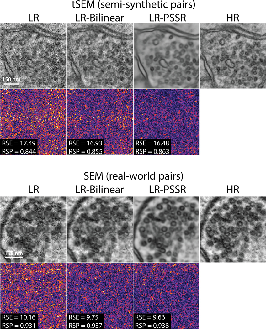
PSNR and SSIM quantification. Two classic image quality metrics, PSNR and SSIM, known for their properties of pixel-level data fidelity and perceptual quality fidelity correspondingly, were used for the quantification of our paired testing image sets. PSNR is inversely correlated with MSE, numerically reflecting the pixel intensity difference between the reconstruction image and the ground truth image, but it is also famous for poor performance when it comes to estimating human perceptual quality. Instead of traditional error summation methods, SSIM is designed to consider distortion factors like luminance distortion, contrast distortion and loss of correlation when interpreting image quality 51 . SNR quantification. SNR was quantified for LSM testing images ( Fig. 4b and Fig. 5a ) by: S N R = I M A X - μ b g σ b g where I M A X represents the maximum intensity value in the image, μ b g and σ b g represent the mean and the standard deviation of the background, respectively 17 . Fourier-Ring-Correlation (FRC) analysis. NanoJ-SQUIRREL 25 was used to calculate image resolution using FRC method on real-world testing examples with two independent acquisitions of fixed samples ( Fig. 2b – c , 4c and Fig. 5b ). Resolution Scaled Error (RSE) and Resolution Scaled Pearson’s coefficient (RSP). NanoJ-SQUIRREL 25 was used to calculate the RSE and RSP for both semi-synthetic and real-world acquired low (LR), bilinear interpolated (LR-Bilinear), and PSSR (LR-PSSR) images versus ground truth high-resolution (HR) images. Difference error maps were also calculated ( Extended Data Fig. 2 , 7 and 10 ). EM Imaging and Analysis tSEM high-resolution training data acquisition.
Tissue from a perfused 7-month old Long
Evans male rat was cut from the left hemisphere, stratum radiatum of CA1 of the hippocampus. The tissue was stained, embedded, and sectioned at 45nm using previously described protocols 52 . Sections were imaged using a STEM detector on a ZEISS Supra 40 scanning electron microscope with a 28kV accelerating voltage and an extractor current of 102μA (gun aperture 30μm). Images were acquired with a 2nm pixel size and a field size of 24576 × 24576 pixels with Zeiss ATLAS. The working distance from the specimen to the final lens was 3.7mm, and the dwell time was 1.2μs. EM testing sample preparation and image acquisition. EM data sets were acquired from multiple systems at multiple institutions for this study. For our testing ground truth data, paired LR and HR images of the adult mouse hippocampal dentate gyrus middle molecular layer neuropil were acquired from ultrathin sections (80nm) collected on silicon chips and imaged in a ZEISS Sigma VP FE-SEM 21 . All animal work was approved by the Institutional Animal Care and Use Committee (IACUC) of the Salk Institute for Biological Studies. Samples were prepared for EM according the NCMIR protocol 53 . Pairs of 4 × 4μm images were collected from the same region at pixels sizes of both 8nm and 2nm using Fibics ATLAS software (InLens detector; 3kV; dwell time, 5.3μs; line averaging, 2; aperture, 30μm; working distance, 2mm). Serial block face scanning electron microscope images were acquired with a Gatan 3View system installed on the ZEISS Sigma VP FE-SEM. Images were acquired using a pixel size of 8nm on a Gatan backscatter detector at 1kV and a current of 221pA. The pixel dwell time was 2μs with an aperture of 30μm and a working distance of 6.81mm. The section thickness was 100nm and the field of view was 24.5 × 24.5μm. Mouse FIB-SEM data sample preparation and image acquisition settings were previously described in the original manuscript the datasets were published 22 . Briefly, the images were acquired with 4nm voxel resolution. We downsampled the lateral resolution to 8nm, then applied our PSSR model to the downsampled data to ensure the proper 8-to-2nm transformation for which the PSSR was trained. Fly FIB-SEM data sample preparation and image acquisition settings were previously described in the original manuscript the datasets were published 54 . Briefly, images were acquired with 10nm voxel resolution. We first upsampled the xy resolution to 8nm using bilinear interpolation, then applied our PSSR model to the upsampled data to ensure the proper 8-to-2nm transformation for which the PSSR model was originally trained. The rat SEM data sample was acquired from an 8-week old male Wistar rat that was anesthetized with an overdose of pentobarbital (75 mg kg −1 ) and perfused through the heart with 5 – 10ml of a solution of 250 mM sucrose 5mM MgCl 2 in 0.02 M phosphate buffer (pH 7.4) (PB) followed by 200 ml of 4% paraformaldehyde containing 0.2% picric acid and 1% glutaraldehyde in 0.1 M PB. Brains were then removed and oblique horizontal sections (50μm thick) of frontal cortex/striatum were cut on a vibrating microtome (Leica VT1200S, Nussloch, Germany) along the line of the rhinal fissure. The tissue was stained and cut to 50nm sections using ATUMtome (RMC Boeckeler, Tucson, USA) for SEM imaging using the protocol described in the original publication for which the data was acquired 55 . The Hitachi Regulus rat SEM data was acquired using a Regulus 8240 FE-SEM with an acceleration voltage of 1.5kV, a dwell time of 3μs, using the backscatter detector with a pixel resolution of 10 × 10nm. We first upsampled the xy resolution to 8nm using bilinear interpolation, then applied our PSSR model to the upsampled data to ensure the proper 8-to-2nm transformation for which the PSSR model was originally trained. EM segmentation and analysis. Image sets generated from the same region of neuropil (LR-Bilinear; LR-PSSR; HR) were aligned rigidly using the ImageJ plugin Linear stack alignment with SIFT 56 . Presynaptic axonal boutons (n = 10) were identified and cropped from the image set. The bouton image sets from the three conditions were then assigned randomly generated filenames and distributed to two blinded human experts for manual segmentation of presynaptic vesicles. Vesicles were identified by having a clear and complete membrane, being round in shape, and of approximately 35nm in diameter. For consistency between human experts, vesicles that were embedded in or attached to obliquely sectioned axonal membranes were excluded. Docked and non-docked synaptic vesicles were counted as separate pools. Vesicle counts were recorded and unblinded and grouped by condition and by expert counter. Linear regression analyses were conducted between the counts of the HR images and the corresponding images of the two different LR conditions (LR-Bilinear; LR-PSSR) to determine how closely the counts corresponded between the HR and LR conditions. Linear regression analysis was also used to determine the variability between counters.
Fluorescence Imaging and Analysis
U2OS cell culture. U2OS cells were purchased from ATCC. Cells were grown in DMEM supplemented with 10% fetal bovine serum at 37 °C with 5% CO 2 . Cells were plated onto either 8-well #1.5 imaging chambers or #1.5 35 mm dishes (Cellvis) coated with 10 μg/mL fibronectin in PBS at 37 °C for 30 minutes prior to plating. 50nm MitoTracker Deep Red or CMXRos Red (ThermoFisher) was added for 30 minutes then washed for at least 30 minutes to allow for recovery time before imaging in FluoroBrite (ThermoFisher) media. Airyscan confocal imaging of U2OS cells. To generate our ground truth training and testing dataset we used a ZEISS Airyscan LSM 880, an advanced confocal microscope that uses a 32-detector array and post-processing pixel reassignment to generate images ~1.7x higher in resolution (~120nm) and ~8x higher SNR than a standard confocal system. All HR ground truth training data were acquired with a 63x objective with at least 2x Nyquist sampling pixel sizes (~50±10nm pixels), then Airyscan processed (deconvolved) using ZEISS Zen software. For the real-world LR test data, we acquired images at 16x lower pixel resolution (~200nm pixel sizes) with a 2.5 AU pinhole on a PMT confocal detector, without any additional image processing. We maintained equal pixel dwell times for the HR versus LR testing acquisitions, resulting in overall 16x shorter exposure times for the LR images. To ensure minimal phototoxicity, we also decreased the laser power for our LR acquisitions by a factor of 4 or 5 (see Tables 1 – 2 for more details), resulting in a net laser dose decrease of ~64–80x (e.g., 5x lower laser power and 16x shorter exposure time yields a 80x lower laser dose). Furthermore, our LR testing data was not deconvolved and used a much larger effective pinhole size than the HR Airyscan ground truth data, resulting in a blurrier image with lower optical resolution. Cells were imaged with a 63× 1.4 NA oil objective on a ZEISS 880 LSM Airyscan confocal system with an inverted stage and heated incubation system with 5% CO 2 control. For both HR and LR images, equal or lower (when indicated) laser power and equal pixel dwell time of ~1 μs/pixel was used. For testing PSSR-MF, at least 10 sequential frames of fixed samples were acquired with high- and low-resolution settings in order to facilitate PSSR-MF processing. Neuron preparation. Primary hippocampal neurons were prepared from E18 rat (Envigo) embryos as previously described. Briefly, hippocampal tissue was dissected from embryonic brain and further dissociated to single hippocampal neuron by trypsinization with Papain (Roche). The prepared neurons were plated on coverslips (Bellco Glass) coated with 3.33μg/mL laminin (Life Technologies) and 20μg/mL poly-L-Lysine (Sigma) at the density of 7.5 × 10 4 cells/cm 2 . The cells were maintained in Neurobasal medium supplemented with B27 (Life Technologies), penicillin/streptomycin and L-glutamine for 7 – 21 days in vitro. Two days before imaging, the hippocampal neurons were transfected with Lipofectamine 2000 (Life Technologies). Temporal consistency analysis. Given a preprocessed time-lapse movie with N total number of frames, the cross-correlation coefficient ( ∅ X i , X i + 1 , i ϵ [ 1 , N ) ) was calculated for two neighboring frames ( X i and X i + 1 ) repeatedly across each movie with a step size of i = 1 ( Fig. 4b ). To ensure comparisons between PSSR output and ground truth data were not biased by high frequency artifacts and noise, each time-lapse was first preprocessed with a Gaussian blur filter ( σ = 5 ) . Fission event detection and analysis. Given fission events cannot be precisely defined across different evaluators, a HR timelapse of mitotracker stained cells was first given to two human experts as a pilot experiment to examine and correct the inspection performance of all experts. Three conditions (LR-Bilinear; LR-PSSR; HR) of the same Airyscan timelapses (n = 6) were then sequentially assigned to two blinded human experts for mitochondria fission event detection. Fission event counts were recorded and unblinded and grouped by condition and by expert counter. Linear regression analyses were conducted between the counts of the HR images and the corresponding images of the two different LR conditions (LR-Bilinear; LR-PSSR) to determine how closely the counts corresponded between the HR and LR conditions. Linear regression analysis was used to determine the variability between counters. Neuronal mitochondria imaging and kymograph analysis. Live-cell imaging of primary neurons was performed using a Zeiss LSM 880 confocal microscope, enclosed in a temperature control chamber at 37 °C and 5% CO 2 , using a 63x (NA 1.4) oil objective in SR-Airyscan mode (i.e. AU virtual pinhole). For low-resolution conditions, images were acquired with a confocal PMT detector with a pinhole size of 2.5 AU at 440 × 440 pixels at 0.5x Nyquist (170nm/pixel) every 270.49ms using a pixel dwell time of 1.2μs and a laser power ranging between 1 – 20 μW. For high-resolution conditions, images were acquired at 1764 × 1764 pixels at 2x Nyquist (~42nm/pixel) every 4.33s using a pixel dwell time of 1.2μs and a laser power of 20μW. Imaging data were collected using Zen Black software. High-resolution images were further processed using Zen Blue’s 2D-SR Airyscan processing. Kymograph analysis of the time-lapse movies were conducted using ImageJ plugin Kymolyzer as described previously 57 . Fluorescence photobleaching quantification. Normalized mean intensity over time was measured using Fiji software. Given a time-lapse movie with N frames, a background region was randomly selected and remained unchanged across frames. The normalized mean intensity ( I - n o r m ( i ) ) can be expressed as: I - n o r m ( i ) = I - i m g ( i ) - I - b g ( i ) M A X ( I - i m g ( i ) - I - b g ( i ) ) , i ∈ 1 , N where i represents the frame index, I - b g ( i ) represents the mean intensity of the selected background region at frame i and I - i m g ( i ) represents the intensity mean of the entire frame i .
Comparing PSSR with other methods Block-matching and 3D filtering
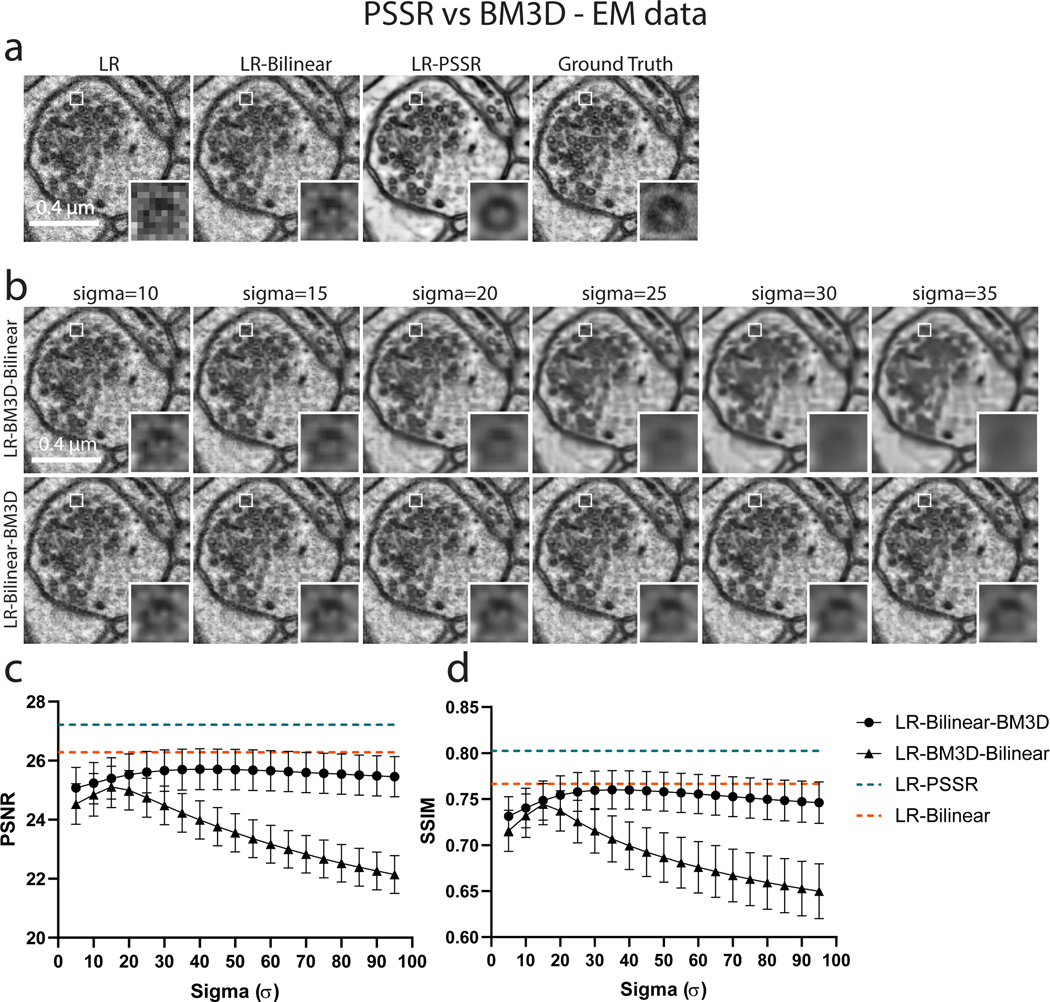
(BM3D) denoising algorithm. We compared PSSR with BM3D, on both EM and fluorescence MitoTracker data. Application of BM3D before (LR-BM3D-Bilinear) and after (LR-Bilinear-BM3D) bilinear upsampling of pixel sizes were both tested. A wide range of Sigma ( σ ∈ 0 , 95 ), the key parameter that defines the assumed zero-mean white Gaussian noise in the images, was thoroughly explored. The exact same test set was used for quantification of PSSR vs. BM3D results.
Content-aware Image Restoration
(CARE) and Rolling Average (RA) methods. A semi-synthetically crappified dataset of MitoTracker data was used to train both CARE and PSSR networks (PSSR-SF and PSSR-MF) in a consistent manner. We applied the trained models to semi-synthetically generated low-resolution testing time-lapses. Testing data were similarly crappified as training data. Five-frame rolling average processing was further applied to CARE and single-frame testing output.
Data Availability
Example training data and pretrained models are included in the GitHub release ( https://github.com/BPHO-Salk/PSSR ). The entirety of our training and testing data sets and data sources are available at Texas Data Repository ( https://doi.org/10.18738/T8/YLCK5A ).
Code Availability
PSSR source code and documentation are available for download on GitHub ( https://github.com/BPHO-Salk/PSSR ) and are free for use under the BSD 3-Clause License. Reporting summary Further information on research design is available in the Life Sciences Reporting Summary linked to this article.
Optimization Methods. Stochastic gradient descent with restarts (SGDR) 47 was implemented. Aside from the benefits we are able to get through classic stochastic gradient descent, SGDR resets the learning rate to its initial value at the beginning of each training epoch and allows it to decrease again following the shape of a cosine function, yielding lower loss with higher computational efficiency.
Comparing PSSR with other methods Block-matching and 3D filtering
(BM3D) denoising algorithm. We compared PSSR with BM3D, on both EM and fluorescence MitoTracker data. Application of BM3D before (LR-BM3D-Bilinear) and after (LR-Bilinear-BM3D) bilinear upsampling of pixel sizes were both tested. A wide range of Sigma ( σ ∈ 0 , 95 ), the key parameter that defines the assumed zero-mean white Gaussian noise in the images, was thoroughly explored. The exact same test set was used for quantification of PSSR vs. BM3D results.
Content-aware Image Restoration
(CARE) and Rolling Average (RA) methods. A semi-synthetically crappified dataset of MitoTracker data was used to train both CARE and PSSR networks (PSSR-SF and PSSR-MF) in a consistent manner. We applied the trained models to semi-synthetically generated low-resolution testing time-lapses. Testing data were similarly crappified as training data. Five-frame rolling average processing was further applied to CARE and single-frame testing output.
Content-aware Image Restoration
(CARE) and Rolling Average (RA) methods. A semi-synthetically crappified dataset of MitoTracker data was used to train both CARE and PSSR networks (PSSR-SF and PSSR-MF) in a consistent manner. We applied the trained models to semi-synthetically generated low-resolution testing time-lapses. Testing data were similarly crappified as training data. Five-frame rolling average processing was further applied to CARE and single-frame testing output.
Supplementary Material 1 1668081_SourceDataFig1 Statistical source data for PSNR, SSIM and FRC resolution plots (panel c-e) 1668081_SourceDataFig2 Statistical source data for PSNR, SSIM and FRC resolution plots of both semi-synthetic (panel b) and real-world testing data (panel c) 1668081_SourceDataFig3 Statistical source data for EM vesicle segmentation analysis plots (panel e) 1668081_SourceDataFig5 Statistical source data for PSNR, SSIM and FRC resolution plots of both semi-synthetic and real-world testing data (panel b) and mitochondrion mobility analysis plots (panel f-i) 1668081_SourceExtDataFig5 Statistical source data for PSNR, SSIM and FRC resolution plots (panel c-e) 1668081_SourceExtDataFig4 Source data for photobleaching intensity plots. 1668081_SourceDataFig4 Statistical source data for flickering quantification plots (panel b), PSNR, SSIM and FRC resolution plots (panel f) and fission event counting plots (panel h-k) 1668081_SourceExtDataFig6 Statistical source data for PSNR and SSIM plots (panel a-b) 1668081_SourceExtDataFig8 Statistical source data for PSNR and SSIM plots (panel c-d) 1668081_SourceExtDataFig3 Statistical source data for PSNR and SSIM plots (panel c-d) 1668081_SuppVideo1 Comparison of high- and low-resolution serial blockface SEM (SBFSEM) 3View acquisition with 2nm and 8nm pixel resolutions. In the 2nm pixel size image stack, high contrast enabled by relatively higher electron doses ensured high-resolution and high SNR, which unfortunately at the same time caused severe sample damage, resulting in a failure to serially section the tissue after imaging the blockface. On the other hand, low-resolution acquisition at 8nm pixel size facilitated serial blockface imaging, but the compromised resolution and SNR made it impossible to uncover finer structures in the sample. 1668081_SuppVideo2 Image restoration achieved by a tSEM-trained PSSR model enables higher resolution SBFSEM imaging. Shown are the lower resolution SBFSEM acquisition input (left) and the PSSR output (right). 1668081_SuppVideo3 Resolution restoration achieved by tSEM-trained PSSR model enables higher resolution FIB-SEM acquisition. Shown are the lower resolution FIB-SEM acquisition input (left) and the PSSR output (right). 1668081_SuppVideo4 PSSR facilitates efficient 3D segmentation and reconstruction. Shown is the rendering of the 3D reconstruction of multiple biological structures using the PSSR processed FIB-SEM stack described in Fig. 3 and Supplementary Movie 3 . Specifically, this reconstruction includes mitochondria (purple), endoplasmic reticulum (yellow), presynaptic vesicles (gray), the postsynaptic neuron’s plasma membrane (blue), the postsynaptic density (red) and the presynaptic neuron’s plasma membrane (green). 1668081_SuppVideo5 Photobleaching and cell stress due to high laser dose during high-resolution live cell imaging. Shown is a 10-minute high-resolution time-lapse movie of a U2OS cell stained with Mitotracker Red imaged with an Airyscan microscope. The live-cell acquisition suffered from photobleaching and phototoxicity as reflected by the steadily decreasing fluorescence intensity over time as well as the swelling and fragmenting mitochondria. Imaging condition: ~35μW laser power, 2s frame rate, 1.15μm pixel size.
1668081_SuppVideo6 PSSR-MF reduces flicker observed in single-frame models
(LR-CARE and LR-PSSR-SF) without loss of spatiotemporal resolution that occurs with rolling frame averaging (LR-CARE-RA and LR-PSSR-SF-RA). Shown is the restoration performance of single-frame PSSR (LR-PSSR-SF), PSSR-SF with 5-frame Rolling Average (LR-PSSR-SF-RA) and 5-frame multi-frame PSSR (LR-PSSR-MF). Rolling Average alleviated the signal flickering observed in single-frame PSSR at the cost of both temporal and spatial resolution. See Extended Data Fig. 4 for more detail. 1668081_SuppVideo7 LR input and 5-frame multi-frame PSSR (LR-PSSR). multi-frame PSSSR restores resolution and SNR to Airyscan equivalent quality with no bleaching and higher imaging speed. Shown are PSSR-MF restoration output (right, ~49nm pixels) and its low-resolution acquisition input (left, ~196nm pixels). The digitally magnified region highlights a mitochondrial fission event much more easily detected in the PSSR output. 1668081_SuppVideo8 Comparison of high-resolution Airyscan and low-resolution confocal time-lapse acquisition of neuronal mitochondria. Corresponding kymographs are also displayed to illustrate the difference in temporal resolution. The Airyscan acquisition has higher spatial resolution but lower temporal resolution due to lower imaging speed, while confocal acquisition gives higher temporal resolution but lower spatial resolution. 1668081_SuppVideo9 Comparison of PSSR (right) versus bilinear interpolation (left). The enlarged region highlights two adjacent mitochondria passing one another in an axon, the process of which was only resolved in PSSR. Line plot shows the normalized fluorescence intensity of the indicated cross-section.
📊 Figures
Extended Data Fig. 1
PSSR Neural Network architecture.
Shown is the ResNet-34 based U-Net architecture. Single-frame PSSR (PSSR-SF) and multi-frame PSSR (PSSR-MF) have 1 or 5 input channels, separately.
Extended Data Fig. 2
NanoJ-SQUIRREL error-maps of EM data.
NanoJ-SQUIRREL was used to calculate the resolution scaled error (RSE) and resolution scaled Pearsonu2019s coefficient (RSP) for both semi-synthetic and real-world acquired low (LR), bilinear interpol...
Extended Data Fig. 3
Comparison of PSSR vs. BM3D on EM data.
PSSR restoration was compared to the Block-matching and 3D filtering (BM3D) denoising algorithm. BM3D was applied to low-resolution real-world SEM images before (LR-BM3D-Bilinear) and after (LR-Biline...
Extended Data Fig. 4
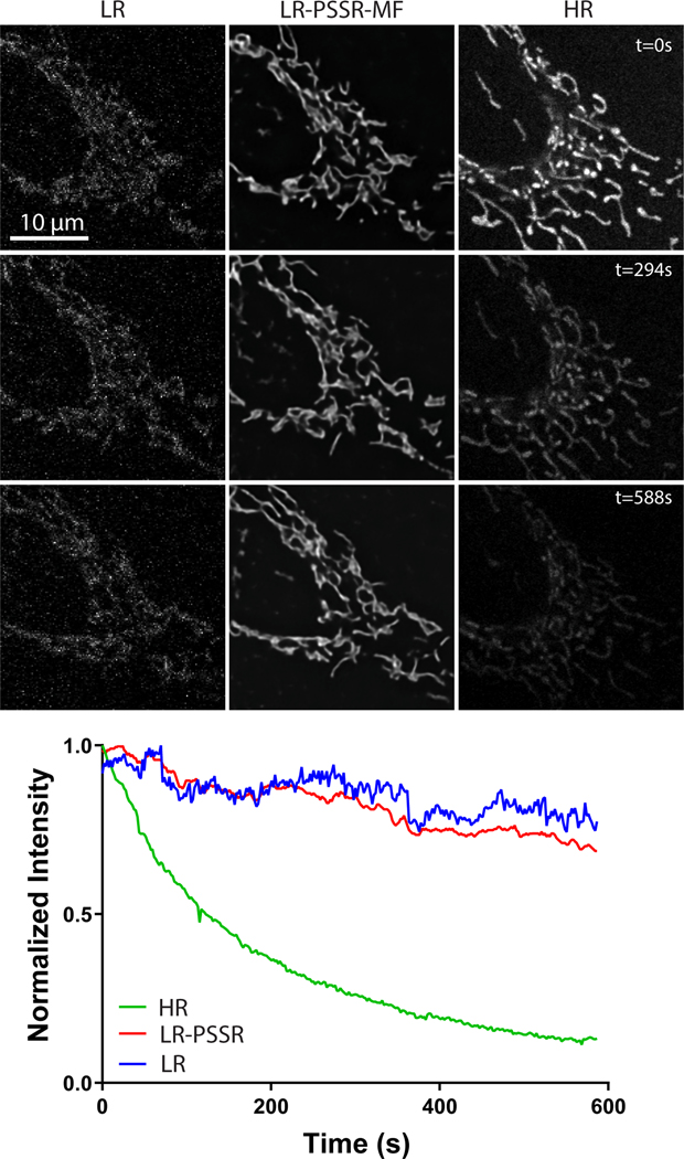
Undersampling significantly reduces photobleaching.
U2OS cells stained with mitotracker were imaged every 2 seconds with the same laser power (2.5u03bcW) and pixel dwell time (~1u03bcs), but with 16x lower resolution (196 u00d7 196nm xy pixel size) tha...
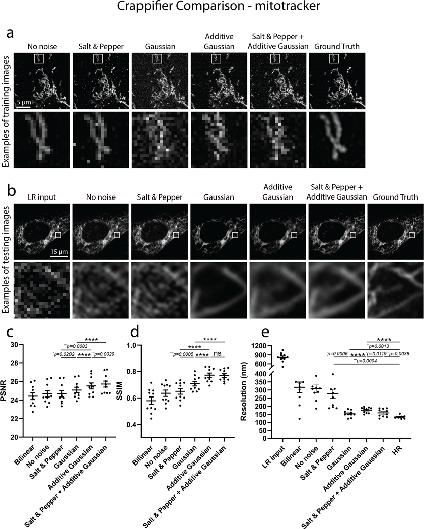
Extended Data Fig. 5
Evaluation of crappifiers with different noise injection on mitotracker data.
Examples of crappified training images, visualized results and metrics (PSNR, SSIM and FRC resolution) of PSSR-SF models that were trained on high- and low-resolution pairs semi-synthetically generate...
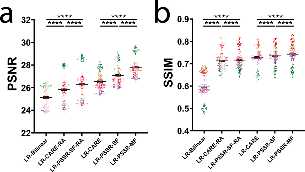
Extended Data Fig. 6
Quantitative comparison of CARE and PSSR-SF with PSSR-MF and Rolling Average (RA) methods for timelapse data.
PSNR ( a ) and SSIM ( b ) quantification show a decrease in accuracy when applying RA to LR-CARE and LR-PSSR-SF, while multi-frame PSSR provides superior performance compared to LR-PSSR-SF and CARE be...
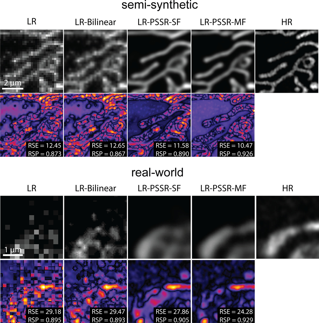
Extended Data Fig. 7
NanoJ-SQUIRREL error-maps of MitoTracker data.
NanoJ-SQUIRREL was used to calculate the resolution scaled error (RSE) and resolution scaled Pearsonu2019s coefficient (RSP) for both semi-synthetic and real-world acquired low (LR), bilinear interpol...
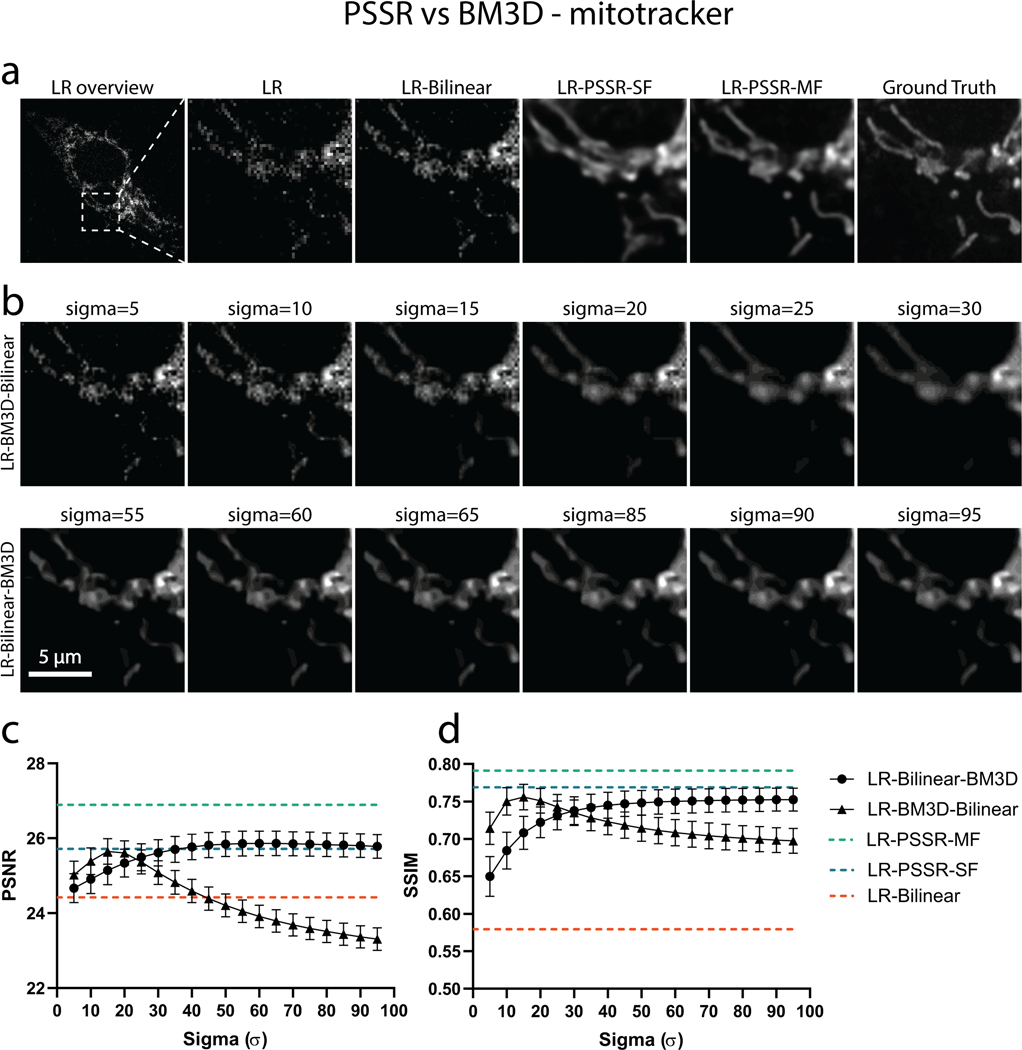
Extended Data Fig. 8
Compare PSSR with BM3D denoising method on mitotracker data.
PSSR restored images was compared to results of applying BM3D denoising algorithm to low-resolution real-world mitotracker images before (LR-BM3D-Bilinear) and after (LR-Bilinear-BM3D) bilinear upsamp...
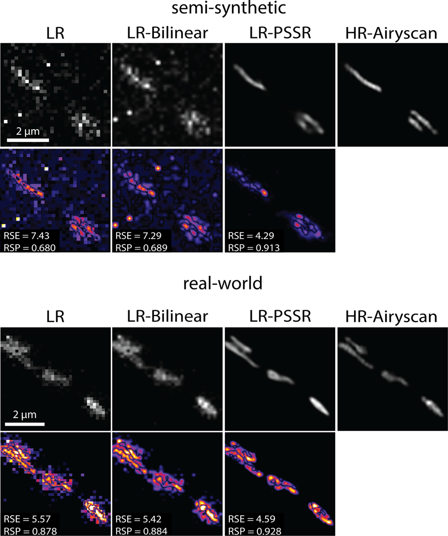
Extended Data Fig. 9
NanoJ-SQUIRREL error-maps of neuronal mitochondria data.
NanoJ-SQUIRREL was used to calculate the resolution scaled error (RSE) and resolution scaled Pearsonu2019s coefficient (RSP) for both semi-synthetic and real-world acquired low (LR), bilinear interpol...
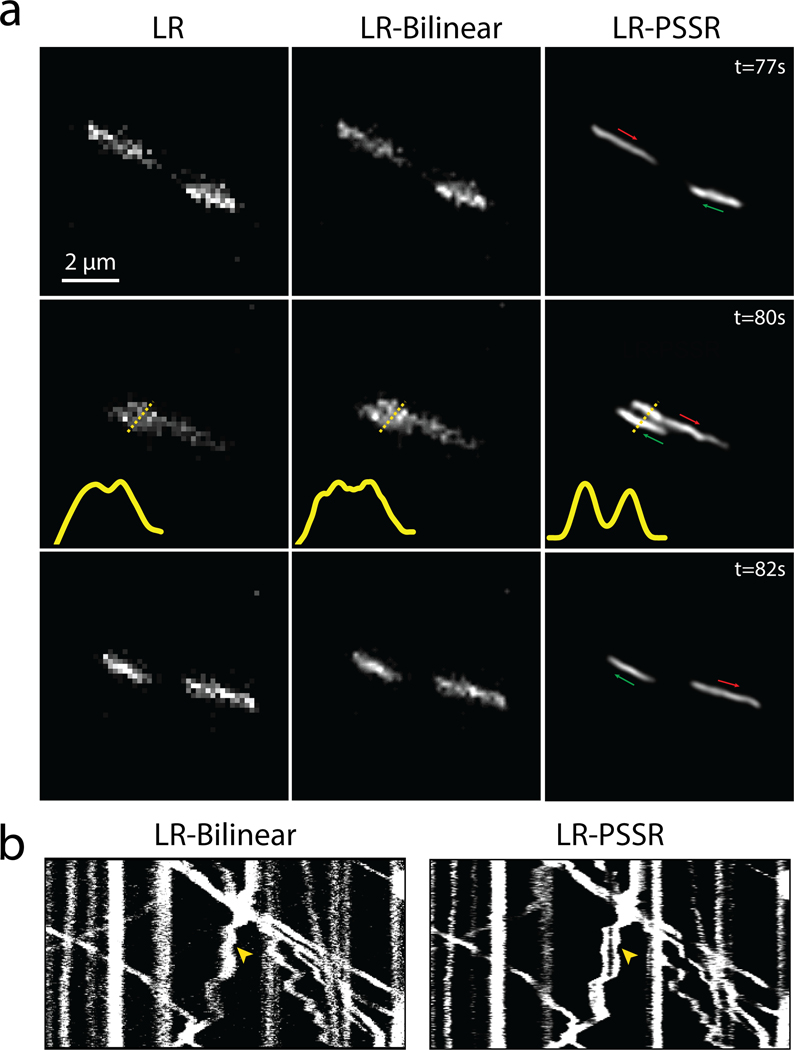
Extended Data Fig. 10
PSSR facilitates detection of mitochondrial motility and dynamics.
Rat hippocampal neurons expressing mito-dsRed were undersampled with a confocal detector using 170nm pixel resolution (LR) to facilitate faster frame rates, then restored with PSSR (LR-PSSR). a, befor...
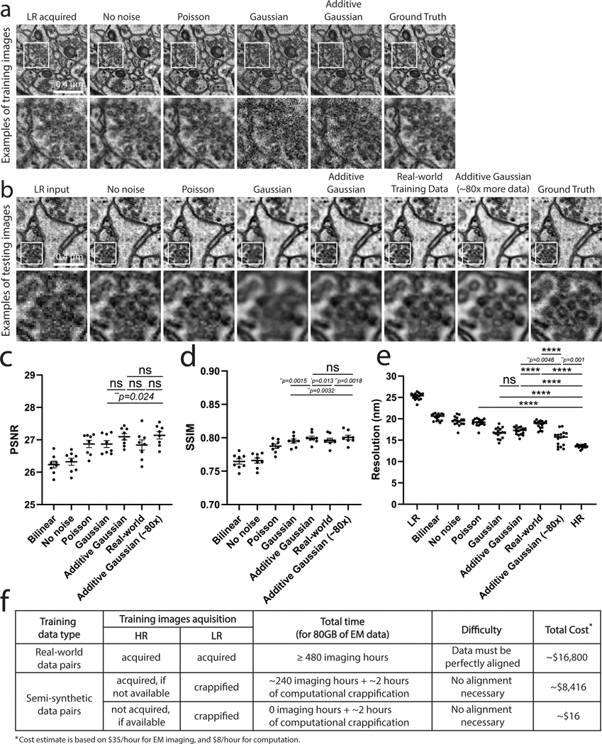
Fig. 1 |
Evaluation of crappifiers with different noise injection on EM data.
a , Different crappifiers applied to high resolution, high SNR images, including u201cNo noiseu201d (no added noise, downsampled pixel size only), u201cPoissonu201d, u201cGaussianu201d, and u201cAddit...
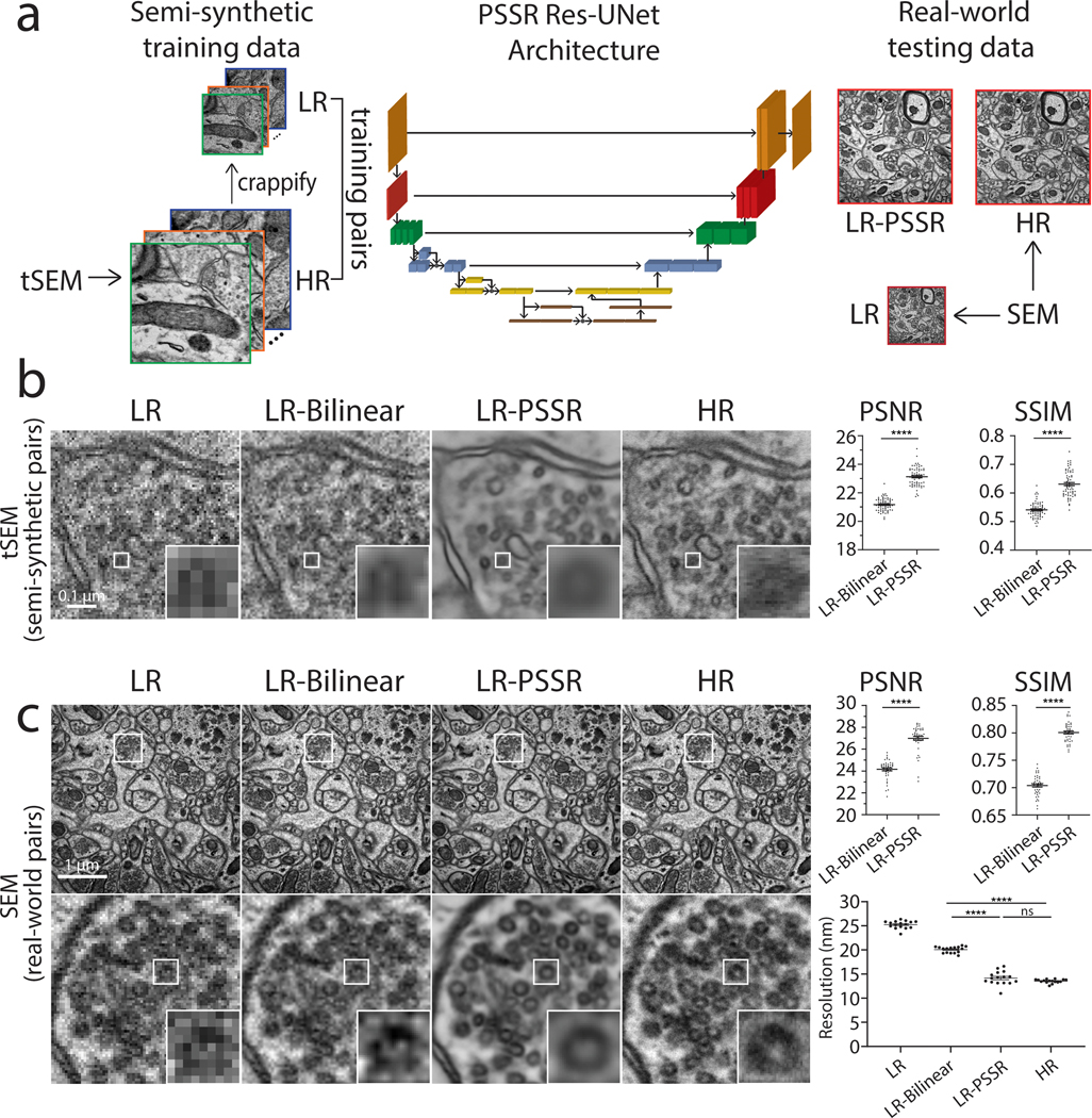
Fig. 2 |
Restoration of semi-synthetic and real-world EM testing data using PSSR model trained on semi-synthetically generated training pairs.
a , Overview of the general workflow. Training pairs were semi-synthetically created by applying a degrading function to the HR images taken from a scanning electron microscope in transmission mode (t...
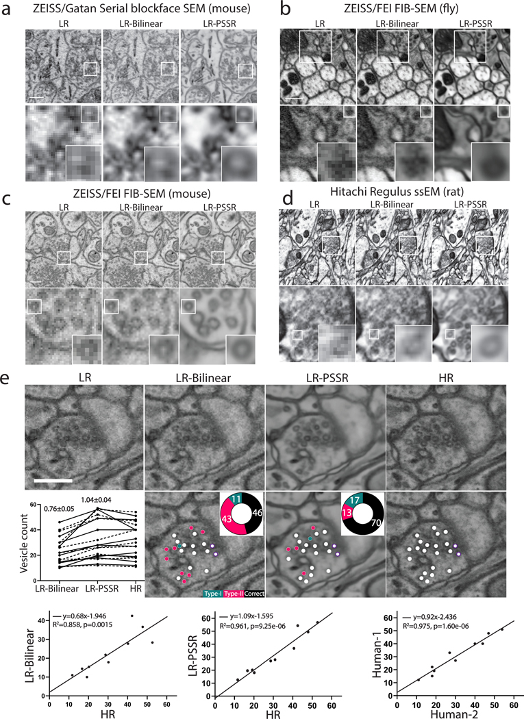
Fig. 3 |
PSSR model is effective for multiple EM modalities and sample types.
Shown are representative low-resolution (LR), bilinear interpolated (LR-Bilinear) and PSSR-restored (LR-PSSR) images from mouse brain sections (n = 75 sections in one image stack, xy dimension 240u00d...
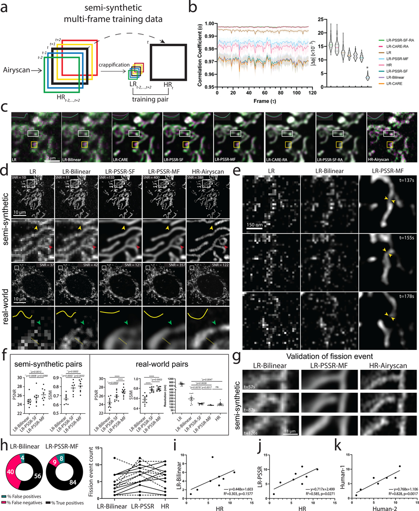
Fig. 4 |
Multi-frame PSSR timelapses of mitochondrial dynamics.
a , Overview of multi-frame PSSR training data generation method. Five consecutive frames ( H R i , i u2208 t - 2 , t + 2 ) from a HR Airyscan time-lapse movie were synthetically crappified to five LR...
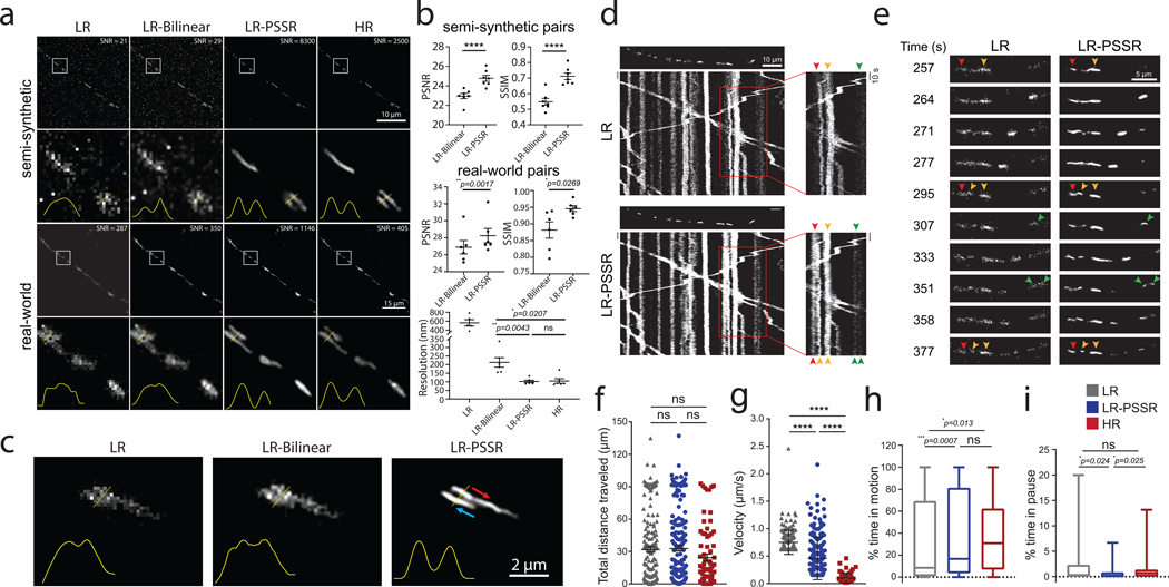
Fig. 5 |
Spatiotemporal analysis of mitochondrial motility in neurons.
PSSR facilitates high spatiotemporal resolution imaging of mitochondrial motility in neurons. a , Comparison of PSSR results (LR-PSSR) versus bilinear interpolation (LR-Bilinear) on semi-synthetic (n ...
Figure images are served from the NIH/NLM PubMed Central Open Access Subset or Europe PMC; copyright remains with the publishers and authors.
💬 Discussion
0 commentsNo comments yet. Be the first to start a discussion!
Leave a Comment