Abstract
AbstractThis work demonstrates and guides how to use a range of state-of-the-art artificial neural-networks to analyse bacterial microscopy images using the recently developed ZeroCostDL4Mic platform. We generated a database of image datasets used to train networks for various image analysis tasks and present strategies for data acquisition and curation, as well as model training. We showcase different deep learning (DL) approaches for segmenting bright field and fluorescence images of different bacterial species, use object detection to classify different growth stages in time-lapse imaging data, and carry out DL-assisted phenotypic profiling of antibiotic-treated cells. To also demonstrate the ability of DL to enhance low-phototoxicity live-cell microscopy, we showcase how image denoising can allow researchers to attain high-fidelity data in faster and longer imaging. Finally, artificial labelling of cell membranes and predictions of super-resolution images allow for accurate mapping of cell shape and intracellular targets. Our purposefully-built database of training and testing data aids in novice users’ training, enabling them to quickly explore how to analyse their data through DL. We hope this lays a fertile ground for the efficient application of DL in microbiology and fosters the creation of tools for bacterial cell biology and antibiotic research.
🔬 Techniques
🔭 Microscopes
🧬 Organisms
✨ Fluorophores
🧪 Sample Preparation
🏭 Microscope Brands
🧪 Reagent Suppliers
📷 Detectors
🔎 Objectives
💻 Software Details
💻 Code & Software
💾 Data Repositories
🏛️ Research Organizations (ROR)
Affiliated research institutions:
📋 Methods
Segmentation of E. coli bright field images E. coli
MG1655 cultures were grown in LB Miller at 37 °C and 220 rounds per minute (rpm) overnight. Working cultures were inoculated 1:200 and grown at 23 °C and 220 rpm to OD600 ~ 0.5–0.8. For time-lapse imaging, cells were immobilised under agarose pads prepared using microarray slides (VWR, catalogue number 732-4826) as described in de Jong et al., 2011 44 . Bright field time series (1 frame/min, 80 min total length) of 10 regions of interest were recorded with an Andor iXon Ultra 897 EMCCD camera (Oxford instruments) attached to a Nikon Eclipse Ti inverted microscope (Nikon Instruments) bearing a motorised XY-stage (Märzhäuser) and an APO TIRF 1.49NA 100x oil objective (Nikon Instruments). To generate the segmentation training data, individual frames from different regions of interest were rescaled using Fiji (2x scaling without interpolation) to allow for better annotation and to match the receptive field of the network. Resulting images were annotated manually using the freehand selection ROI tool in Fiji. For quality control, a test dataset of 15 frames was generated similarly. Contrast was enhanced in Fiji and images were either converted into 8-bit TIFF (CARE, U-Net, StarDist) or PNG format (pix2pix). To track cells during their release from stationary phase, we immobilised cells from an ON culture as described above. Time series of multiple positions were recorded at 2 min interval (40 min in total). To account for the small size of the cells, we used an additional tube lens (1.5x) to reduce the pixel size to 106 nm. To obtain the training dataset, we recorded stationary phase cells directly after immobilization and additionally annotated selected individual frames from the time series.
Show full methods section
Segmentation of E. coli bright field images E. coli
MG1655 cultures were grown in LB Miller at 37 °C and 220 rounds per minute (rpm) overnight. Working cultures were inoculated 1:200 and grown at 23 °C and 220 rpm to OD600 ~ 0.5–0.8. For time-lapse imaging, cells were immobilised under agarose pads prepared using microarray slides (VWR, catalogue number 732-4826) as described in de Jong et al., 2011 44 . Bright field time series (1 frame/min, 80 min total length) of 10 regions of interest were recorded with an Andor iXon Ultra 897 EMCCD camera (Oxford instruments) attached to a Nikon Eclipse Ti inverted microscope (Nikon Instruments) bearing a motorised XY-stage (Märzhäuser) and an APO TIRF 1.49NA 100x oil objective (Nikon Instruments). To generate the segmentation training data, individual frames from different regions of interest were rescaled using Fiji (2x scaling without interpolation) to allow for better annotation and to match the receptive field of the network. Resulting images were annotated manually using the freehand selection ROI tool in Fiji. For quality control, a test dataset of 15 frames was generated similarly. Contrast was enhanced in Fiji and images were either converted into 8-bit TIFF (CARE, U-Net, StarDist) or PNG format (pix2pix). To track cells during their release from stationary phase, we immobilised cells from an ON culture as described above. Time series of multiple positions were recorded at 2 min interval (40 min in total). To account for the small size of the cells, we used an additional tube lens (1.5x) to reduce the pixel size to 106 nm. To obtain the training dataset, we recorded stationary phase cells directly after immobilization and additionally annotated selected individual frames from the time series.
Data pre- and post-processing for cell segmentation using the multi-label
U-Net notebook In order to improve segmentation performance, we employed a U-Net that is trained on semantic segmentations of both cell cytosol and boundaries. To generate the respective training data, annotated cells were filled with a grey value of 1, while cell boundaries were drawn with a grey value of 2 and a line thickness of 1. Together with the fluorescence image, this image was used as network input during training. During post-processing, cell boundaries were subtracted from predicted cell segmentations, followed by thresholding and marker-based watershed segmentation (Fiji plugin “MorpholibJ”) 78 . Pre- and post-processing routines are provided as Fiji macros and can be downloaded from the DeepBacs github repository. Segmentation of S. aureus bright field and fluorescence images For S. aureus time-lapse experiments overnight cultures of S. aureus strain JE2 were back-diluted 1:500 in tryptic soy broth (TSB) and grown to mid-exponential phase (OD 600 = 0.5). One millilitre of the culture was incubated for 5 min (at 37 °C) with the membrane dye Nile Red (5 µg/ml, Invitrogen), washed once with phosphate buffered saline (PBS), subsequently pelleted and resuspended in 20 µl PBS. One microlitre of the labelled culture was then placed on a microscope slide covered with a thin layer of agarose (1.2% (w/v) in 1:1 PBS/TSB solution). Time-lapse images were acquired every 25 s (for differential interference contrast (DIC)) and 5 min (for fluorescence images) by structured illumination microscopy (SIM) or classical diffraction limited widefield microscopy in a Deltavision OMX system (with temperature and humidity control, 37 °C). The images were acquired using 2 PCO Edge 5.5 sCMOS cameras (one for DIC, one for fluorescence), an Olympus 60×1.42NA Oil immersion objective (oil refractive index 1.522), Cy3 fluorescence filter sets (for the 561 nm laser) and DIC optics. Each time-point results from a Z-stack of 3 epifluorescence images using either the 3D-SIM optical path (for SIM images) or classical widefield optical path (for non-super-resolution images). These stacks were acquired with a Z step of 125 nm in order to use the 3D-SIM-reconstruction modality (for the SIM images) of Applied Precision’s softWorx software (AcquireSRsoftWoRx v7.0.0 release RC6), as this provides higher quality reconstructions. A 561 nm laser (100 mW) was used at 11–18 W cm −2 with exposure times of 10–30 ms. For single-acquisition S. aureus experiments, sample preparation and image acquisition were performed as mentioned above but single images were acquired. To generate the training dataset for StarDist segmentation, individual channels were separated and pre-processed using Fiji 9 , 43 . Nile Red fluorescence images were manually annotated using ellipsoid selections to approximate the S. aureus cell shape. Resulting ROIs were used to generate the required ROI map images (using the “ROI map” command included in the Fiji plugin LOCI) in which each individual cell is represented by an area with a unique integer value. Training images (512 × 512 px²) were further split into 256 × 256 px² images, resulting in 28 training images pairs. 5 full field-of-view test image pairs were provided for model quality control. For segmentation dataset of S. aureus bright field images, we used the ROI masks created for Nile Red fluorescence image segmentation, as both images were acquired in parallel.
Segmentation of live B. subtilis cells B. subtilis cells expressing
FtsZ-GFP (strain SH130, PY79 Δhag ftsZ::ftsZ-gfp-cam) were prepared as described in Whitley et al., 2021 47 . Strains were taken from glycerol stocks kept at −80 °C and streaked onto nutrient agar (NA) plates containing 5 µg/ml chloramphenicol then grown overnight at 37 °C. Liquid cultures were started by inoculating time-lapse medium (TLM) (de Jong et al., 2011) 44 with a single colony and growing overnight at 30 °C with 200 rpm agitation. The following morning, cultures were diluted into chemically defined medium (CDM) containing 5 µg/ml chloramphenicol to OD 600 = 0.1, and grown at 30 °C until the required optical density was achieved 47 . All imaging was done on a custom built, 100X inverted microscope. A 100x TIRF objective (Nikon CFI Apochromat TIRF 100XC Oil), a 200 mm tube lens (Thorlabs TTL200) and Prime BSI sCMOS camera (Teledyne Photometrics) were used achieving an imaging pixel size of 65 nm/pixel. Cells were illuminated with a 488 nm laser (Obis) and imaged using a custom ring-TIRF module operated in ring-HiLO 79 . A pair of galvanometer mirrors (Thorlabs) spinning at 200 Hz provides uniform, high SNR illumination. The raw data analysed here were acquired and analysis of that raw data presented in Whitley et al., 2021 47 . These data have now been reanalysed using cell segmentation methods discussed. Slides were prepared as described previously. Molten 2% agarose made with CDM was poured into gene frames (Thermo Scientific) to form flat agarose pads, then cut down to thin 5 mm strips. 0.5 µl of cell culture grown to mid-exponential phase (OD 600 = 0.2–0.3) was spotted onto the agarose and allowed to absorb (~30 s). A plasma-cleaned coverslip was then placed atop the gene frame and sealed in place. Before imaging, the prepared slides were then pre-warmed inside the microscope body at least 15 min before imaging. Time-lapse images were then taken in TIRF using a custom built 100x inverted microscope. Images were taken at 1 s exposure, 1 frame/min at 1–8 W/cm 2 47 . Videos were denoised using ImageJ plugin PureDenoise 35 then lateral drift was corrected using StackReg 80 . To create the training dataset, 10 frames were extracted from each time-lapse ~10 frames apart. This was to ensure sufficient difference between the images used for training. Ground truth segmentation maps were generated by manual annotation of cells in each frame using the Fiji/ImageJ LabKit plugin lab ( https://github.com/juglab/imglib2-labkit ). This process assigns a distinct integer to all pixels within a cell region, and background pixels are labelled 0. A total of 4,672 cells were labelled across 80 distinct frames to create the final training dataset.
Confocal imaging for denoising of E. coli time series
E. coli strain CS01 carrying a chromosomal H-NS-mScarlet-I protein fusion (parental strain NO34) was grown in LB Lennox at 25 °C and shaking at 220 rpm. To generate the training dataset, cells were fixed chemically using a mixture of 2% formaldehyde and 0.1% glutaraldehyde. Fixed or live cells were immobilised under agarose pads poured into gene frames following the protocol by de Jong et al. 44 . Imaging was performed on a commercial Leica SP8 confocal microscope (Leica Microsystems) bearing a 1.40 NA 63x oil immersion objective (Leica Microsystems). To increase optical sectioning, the pinhole size was set to 0.5 airy units and 512 × 512 px² confocal images (45 nm pixel size) were recorded. Emission was detected with HyD detectors in standard operation mode (gain 100, detection window 570–650 nm). For the training dataset, a two-channel image of the same structure was recorded in frame sequential mode using different settings for low (0.03% 561 nm laser light, no averaging) and high SNR images (0.1% 561 nm laser light, 4x line averaging), respectively. For live-cell time series, the field of view was reduced to 256 × 256 px² to allow for fast acquisition of high SNR images at ~0.8 Hz. Low SNR time series were recorded at similar frame rate by including a lag time. Similar settings were used for the MreB denoising dataset, except that sfGFP was excited with 488 nm and fluorescence was detected between 495 nm and 560 nm. To increase optical sectioning even further to optimized observation of processive MreB movement, the pinhole size was set to 0.3 airy units.
B. subtilis VerCINI microscopy
The raw data analysed here were acquired and analysis of that raw data is presented in Whitley et al. 2021 47 . These data have now been reanalysed using the denoising methods described. Silicone micropillar wafers were nanofabricated and used to prepare agarose microholes as described in Whitley et al., 2021 47 . Molten 6% agarose was poured onto the silicone micropillars and allowed to set, forming an agarose pad punctured with microscopic holes. The agarose pad was then transferred into a gene frame, and agarose surrounding the micro-hole array was cut away. Concentrated liquid cell culture at mid-exponential phase (OD 600 = 0.4) was loaded onto the pad and centrifugation using an Eppendorf 5810 centrifuge with MTP/Flex buckets loaded individual cells into the microholes. The pad was then washed to remove unloaded cells. This repeated several times until a sufficient level cell loading was achieved. Cells were imaged at 1 frame/second with continuous exposure for 2 min at 1–8 W/cm 2 47 . Image denoising was performed using the ImageJ plugin PureDenoise 35 and lateral drift was then corrected using StackReg 80 .
E. coli cell cycle classification
Classification of rod-shaped, dividing and microcolonies was performed using the time series described in section ‘ Segmentation of E. coli bright field images’ . Individual frames from several time series were used for training. To generate the training dataset, individual frames spread over the entire time series (typically frames 1, 15, 30, 55 and 80) were converted into PNG format. For the large field-of-view model, the entire image was used, while images were split into 4 regions of 256 × 256 px² size for the small field-of-view model. Images were annotated using LabelImg 49 . The final training dataset contained 25 (100 for small field-of-view) annotated patches, and dataset size was increased 4x during training using data augmentation implemented in the ZeroCostDL4Mic YOLOv2 notebook (rotation and flipping).
E. coli antibiotic phenotyping
E. coli strain NO34 55 was grown in LB at 32 °C shaking at 220 rpm overnight. Working cultures were inoculated 1:200 in fresh LB and grown to mid-exponential phase and antibiotics were added at the concentration and for the time listed in Supplementary Table 7 . Antibiotic stock solutions were prepared freshly 5-10 min before use. Cells were fixed using a mixture of 2% formaldehyde and 0.1% glutaraldehyde, quenched using 0.1% sodium borohydrate (w/v) in PBS for 3 min and immobilised on PLL-coated chamber slides (see Spahn et al. 2018 for details 64 ). Nucleoids were stained using 300 nM DAPI for 15 min. After three washes with PBS, 100 nM Nile Red in PBS was added to the chambers and confocal images were recorded with a commercial LSM710 microscope (Zeiss, Germany) bearing a Plan-Apo 63x oil objective (1.4 NA) and using 405 nm (DAPI) and 543 nm (Nile Red) laser excitation in sequential mode. Images (800 × 800 px²) were recorded with a pixel size of 84 nm, 16-bit image depth, 16.2 µs pixel dwell time, 2x line averaging and 1 airy unit pinhole size. Four to eight confocal images were used to generate the training dataset, depending on the cell count per image (for example, only few cells are present per image for nalidixate-treated cells, while many cells were present for chloramphenicol treatment). Each image was converted to PNG format, split into 4 non-overlapping patches (400 × 400 px²) and patches were annotated online using makesense.ai 81 . Annotations were exported in PASCAL VOC format. Next to the 5 antibiotic treatments and control conditions, vesicles and partially attached cells were added as additional classes (“Vesicles” and “Oblique”, respectively), resulting in a total of eight classes. Synthetic test data was generated by randomly stitching 200 × 200 px² patches of different drug treatments and the control condition. Small patches were manually cropped from images that were not seen by the network during the training. In total, 32 test images were generated this way and annotated online using makesense.ai 81 as described above. Additionally, 400 × 400 px² image patches of previously unseen images (drug treatments and control) were annotated using LabelImg 49 . Artificial labelling of E. coli membranes PAINT super-resolution images of E. coli membranes were recorded as described elsewhere 64 . In brief, cells were grown in LB at 37 °C and 220 rpm, fixed in mid-exponential phase (OD 600 = 0.5) using a mixture of 2% formaldehyde and 0.1% glutaraldehyde, immobilised on poly-L-Lysine coated chamber slides and permeabilised with 0.5% TX-100 in PBS for 30 min. 400 pM Nile Red in PBS was added and PAINT time series (6,000–10,000 frames) were recorded on a custom built setup for single-molecule detection (Nikon Ti-E body equipped with a 100x Plan Apo TIRF 1.49 NA oil objective) using 561 nm excitation (~1 kW/cm²) or a commercial N-STORM system with a similar objective and imaging parameters. Two image datasets were recorded using either a 1x or 1.5x tube lens (158 and 106 nm pixel size, respectively). PAINT images were reconstructed using Picasso v.0.2.8 and v.0.3.3 82 and exported at different magnifications (8x for 158 nm pixel [19.8 nm/px] and 6x for 106 nm pixel size [17.7 nm/px]). Corresponding bright field images were scaled similarly in Fiji without interpolation and registered with the PAINT image. Multiple 512 × 512 px² image patches were extracted from these images and used for model training. For artificial labelling in drug-treated cells, cells were exposed to the following antibiotics: 100 µg/ml rifampicin for 10 min, 50 µg/ml Chloramphenicol for 60 min, 2 µg/ml Mecillinam for 60 min. Further sample preparation and imaging was performed similar to untreated cells. Prediction of membrane SIM images in live E. coli and S. aureus cells For widefield-to-SIM prediction experiments overnight cultures of E. coli strain DH5α were back-diluted 1:500 in LB and grown to mid-exponential phase (OD 600 = 0.3). One millilitre of the culture was incubated for 10 min (at 37 °C) with the membrane dye FM5-95 (10 µg/ml, Invitrogen), washed once with PBS, subsequently pelleted and resuspended in 10 µl PBS. One microliter of the labelled culture was then placed on a microscope slide covered with a thin layer of agarose (1.2% (w/v) in 1:1 PBS/LB solution). Image acquisition was performed as mentioned in section “Segmentation of S. aureus bright field and fluorescence images”. To generate the paired training dataset for super-resolution prediction, raw SIM images were averaged to obtain the diffraction limited widefield image, while the in-focus plane of the SIM reconstruction was used as corresponding high-resolution image. The dataset was curated by removing defocused images and images with low signal resulting in reconstruction artefacts. In total, 55 training and five test image pairs were used for E. coli . For S. aureus , this resulted in 94 training and five test image pairs. Data augmentation As a general strategy to increase training dataset sizes, we used data augmentation 22 , 83 for all DL learning tasks performed in this study using mostly image rotation and flipping. Calculation of the multiscale structural similarity index (SSIM) Performance of several DL approaches (e.g. CARE) was accessed by calculating the multiscale structural similarity index (here denoted as SSIM) between the source/predicted image and the ground truth image 54 (see Supplementary Note 1 ). Since background is suppressed efficiently by most networks and is thus over-proportionally contributing to the average per-image SSIM value (leading to an over-optimistic value), we determined the SSIM only within the outlines of bacterial cells. For this, ROIs were generated in Fiji by thresholding the high SNR image or time series average image. For denoising of live-cell time series lacking ground truth data (e.g. N2V), we determined the SSIM value over time by comparing each image frame to the subsequent image frame of the time series (thus termed subsequent-frame SSIM). A low SSIM value thus depicts a high frame-to-frame variation. Tracking analysis using TrackMate To track exponentially growing cells (Supplementary Video 3 ) and cells transitioning from stationary to lag phase (Supplementary Video 4 ), we used the ‘mask image detector’ in DL-capable version of TrackMate 46 . No thresholding was used on the detected labels and the LAP tracker was used with 10 px linking distance and segment gap closing (5 px). To track MreB filaments, we used the LoG detector with a radius of 0.25 µm (0.5 µm diameter) and varying thresholds for low SNR, high SNR and denoised time series. Linking distance was set to 0.2 µm using the simple LAP tracker.
SQUIRREL analysis
To access artefacts in super-resolution prediction from widefield data we used the SQUIRREL algorithm implemented in the Fiji NanoJ plugin 66 , 84 . This way, the predictions of 5 WF images and the respective SIM ground truth images were analysed. SQUIRREL calculates a diffraction limited image from super-resolution images to compare them with the corresponding low-resolution ground truth image. Resulting error maps give rise to reconstruction and in this case also prediction artefacts.
Statistics and reproducibility
For the majority of datasets, multiple images or time series were recorded in a single imaging session. It was ensured that the acquired data is representative by the different expert laboratories contribution to this work. For object detection (drug-treated cells) and artificial labelling (super-resolution), images from 2–3 independent experiments were included in the training and test dataset. Information about the number of training images and/or cell count per image is provided in the Supplementary Information and the Supplementary Data 1 . The latter also includes the individual values used for statistical analysis. Reporting summary Further information on research design is available in the Nature Research Reporting Summary linked to this article.
Supplementary information Peer Review File Supplementary Information Description of Additional Supplementary Files Supplementary Video 1 Supplementary Video 2 Supplementary Video 3 Supplementary Video 4 Supplementary Video 5 Supplementary Video 6 Supplementary Video 7 Supplementary Video 8 Supplementary Video 9 Supplementary Video 10 Supplementary Video 11 Supplementary Data 1 Reporting Summary
📊 Figures
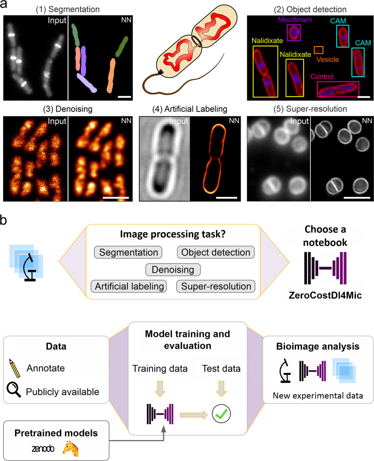
Fig. 1
Overview of the DL tasks and datasets used in DeepBacs.
a We demonstrate the capabilities of DL in microbiology for segmentation (1), object detection (2), denoising (3), artificial labelling (4) and prediction of super-resolution images (5) of microbial m...
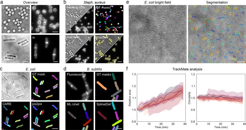
Fig. 2
Segmentation of bacterial images using open-source deep learning approaches.
a Overview of the datasets used for image segmentation. Shown are representative regions of interest for (i) S. aureus bright field and (ii) fluorescence images (Nile Red membrane stain), (iii) E. col...
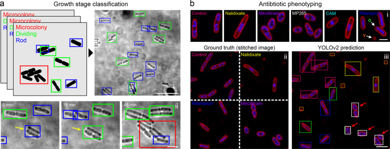
Fig. 3
DL-based object detectionu00a0and classification.
a A YOLOv2 model was trained to detect and classify different growth stages of live E. coli cells (i). u201cDividingu201d cells (green bounding boxes) show visible septation, the class u201cRodu201d (...
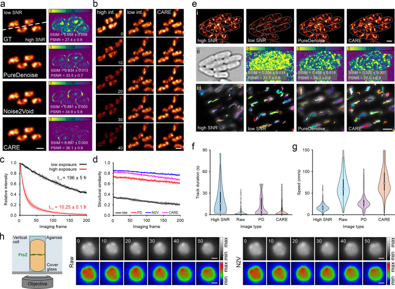
Fig. 4
Image denoising for improved live-cell imaging in bacteriology.
a Low and high signal-to-noise ratio (SNR) image pairs (ground truth, GT) of fixed E. coli cells, labelled for H-NS-mScarlet-I. Denoising was performed with PureDenoise (parametric approach), Noise2Vo...
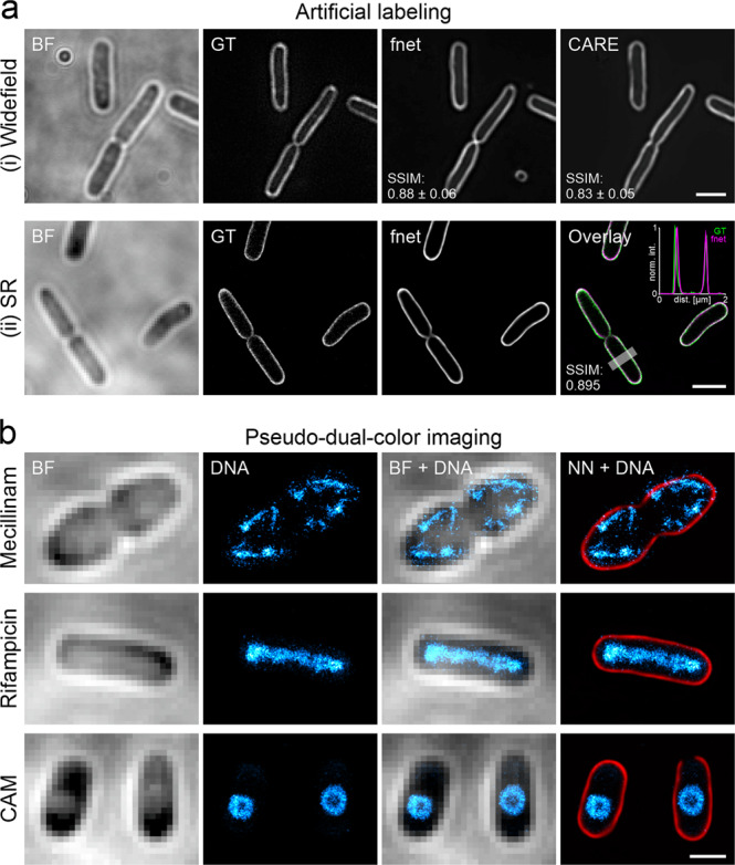
Fig. 5
Artificial labelling of E. coli membranes.
a fnet and CARE predictions of diffraction-limited (i) and PAINT super-resolution (SR) (ii) membrane labels obtained from bright field (BF) images. GTu2009=u2009ground truth. Values represent averages...
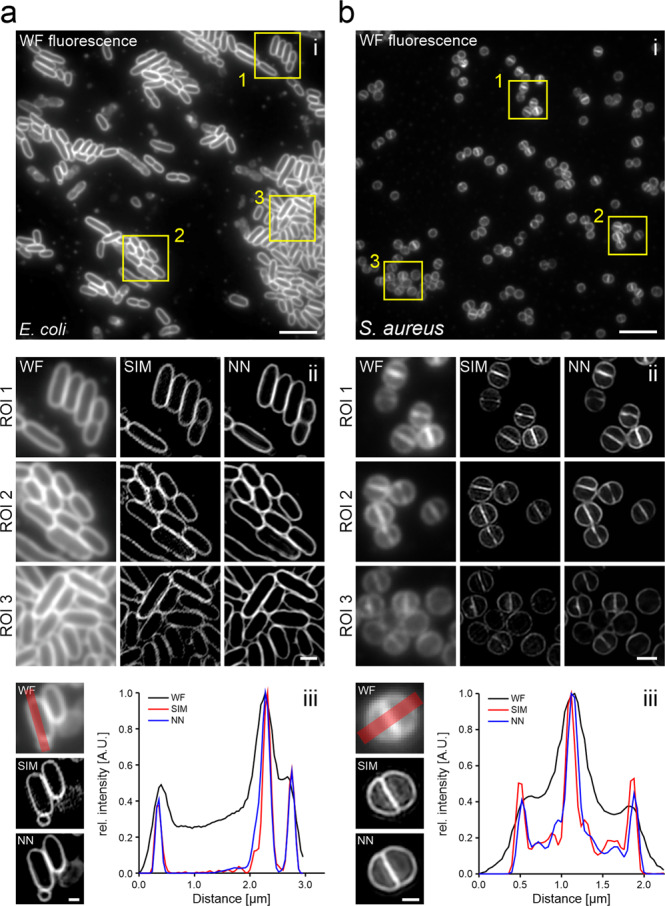
Fig. 6
Prediction of SIM images from widefield fluorescence images.
Widefield-to-SIM image transformation was performed with CARE for a live E. coli (FM5-95) and b S. aureus (Nile Red) cells. Shown are diffraction-limited widefield images (i) and the magnified regions...
Figure images are served from the NIH/NLM PubMed Central Open Access Subset or Europe PMC; copyright remains with the publishers and authors.
💬 Discussion
0 commentsNo comments yet. Be the first to start a discussion!
Leave a Comment