Abstract
Our knowledge of transcriptional heterogeneities in epithelial stem and progenitor cell compartments is limited. Epidermal basal cells sustain cutaneous tissue maintenance and drive wound healing. Previous studies have probed basal cell heterogeneity in stem and progenitor potential, but a comprehensive dissection of basal cell dynamics during differentiation is lacking. Using single-cell RNA sequencing coupled with RNAScope and fluorescence lifetime imaging, we identify three non-proliferative and one proliferative basal cell state in homeostatic skin that differ in metabolic preference and become spatially partitioned during wound re-epithelialization. Pseudotemporal trajectory and RNA velocity analyses predict a quasi-linear differentiation hierarchy where basal cells progress from Col17a1Hi/Trp63Hi state to early-response state, proliferate at the juncture of these two states, or become growth arrested before differentiating into spinous cells. Wound healing induces plasticity manifested by dynamic basal-spinous interconversions at multiple basal transcriptional states. Our study provides a systematic view of epidermal cellular dynamics, supporting a revised "hierarchical-lineage" model of homeostasis.
🔬 Techniques
🔭 Microscopes
💻 Software
✨ Fluorophores
🧪 Sample Preparation
🔬 Cell Lines
🏭 Microscope Brands
🧪 Reagent Suppliers
🔴 Lasers
🎨 Filters
💻 Software Details
💻 Code & Software
💾 Data Repositories
🏛️ Research Organizations (ROR)
Affiliated research institutions:
📋 Methods
LEAD CONTACT AND MATERIALS AVAILABILITY
Further information and requests for resources and reagents should be directed to and will be fulfilled by the Lead Contact, Xing Dai ( xdai@uci.edu ). This study did not generate new unique reagents.
EXPERIMENTAL MODEL AND SUBJECT DETAILS K14-Cre transgenic mice
(C57BL/6J background) have been previously described ( Andl et al., 2004 ). ROSA mTmG (C57BL/6J background) and wild-type C57BL/6J mice are from the Jackson Laboratory (Stock #s 007576 and 000664, respectively). Seven-week old female mice were used for the studies. All maintenance, care, and experiments have been approved and abide by regulatory guidelines of the International Animal Care and Use Committee (IACUC) of the University of California, Irvine. METHOD DETAILS Wounding For single cell experiments, 7-week-old (p49, telogen) female C57BL/6J mice were anesthetized using isoflurane (Primal Healthcare; NDC-66794-017-25), backs shaved, and then a 6-mm punch (Integra; 33-36) was used to generate a full-thickness wound on each side of the mouse. Wounds were collected 4 days later for analysis. For FLIM-related wounding experiments, 7 week-old female K14-Cre; ROSA mTmG mice (C57BL/6J background) were anesthetized using isoflurane, backs shaved, and Nair was applied to the backs of the shaved mice for complete hair removal. A 6-mm punch was used to generate a full-thickness wound on each side of the mouse. Four days after wounding, the wound and surrounding un-wounded skin regions were excised (approximately 1.5 cm in diameter with surgical scissors) for analysis. Single cell isolation for scRNA-Seq For UW back skin, 7-week-old (p49, telogen) female C57BL/6J mice were shaved, back skin removed, fat scrapped off, and then skin was minced into pieces less than 1 mm in diameter. For WO back skin, skin was removed, large pieces of fat attached to underside of the wound were carefully removed, a 10-mm punch (Acuderm; 0413) was then used to capture the wound and a portion of unwounded skin adjacent to the wound. The wounds were then minced into pieces less than 1 mm in diameter. The minced samples were placed in 15-mL conical tubes and digested with 10 mL of collagenase mix [0.25% collagenase (Sigma; C9891), 0.01M HEPES (Fisher; BP310), 0.001M sodium pyruvate (Fisher; BP356), and 0.1 mg/mL DNase (Sigma; DN25)]. Samples were incubated at 37°C for 2 hours with rotation, and then filtered through 70-μm and 40-μm filters, spun down, and resuspended in 2% FBS. Cells were stained with SytoxBlue (Thermo Fisher; S34857) as per manufacturer’s instructions and live cells (SytoxBlue-negative) were sorted using BD FACSAria Fusion Sorter.
Show full methods section
LEAD CONTACT AND MATERIALS AVAILABILITY
Further information and requests for resources and reagents should be directed to and will be fulfilled by the Lead Contact, Xing Dai ( xdai@uci.edu ). This study did not generate new unique reagents.
EXPERIMENTAL MODEL AND SUBJECT DETAILS K14-Cre transgenic mice
(C57BL/6J background) have been previously described ( Andl et al., 2004 ). ROSA mTmG (C57BL/6J background) and wild-type C57BL/6J mice are from the Jackson Laboratory (Stock #s 007576 and 000664, respectively). Seven-week old female mice were used for the studies. All maintenance, care, and experiments have been approved and abide by regulatory guidelines of the International Animal Care and Use Committee (IACUC) of the University of California, Irvine. METHOD DETAILS Wounding For single cell experiments, 7-week-old (p49, telogen) female C57BL/6J mice were anesthetized using isoflurane (Primal Healthcare; NDC-66794-017-25), backs shaved, and then a 6-mm punch (Integra; 33-36) was used to generate a full-thickness wound on each side of the mouse. Wounds were collected 4 days later for analysis. For FLIM-related wounding experiments, 7 week-old female K14-Cre; ROSA mTmG mice (C57BL/6J background) were anesthetized using isoflurane, backs shaved, and Nair was applied to the backs of the shaved mice for complete hair removal. A 6-mm punch was used to generate a full-thickness wound on each side of the mouse. Four days after wounding, the wound and surrounding un-wounded skin regions were excised (approximately 1.5 cm in diameter with surgical scissors) for analysis. Single cell isolation for scRNA-Seq For UW back skin, 7-week-old (p49, telogen) female C57BL/6J mice were shaved, back skin removed, fat scrapped off, and then skin was minced into pieces less than 1 mm in diameter. For WO back skin, skin was removed, large pieces of fat attached to underside of the wound were carefully removed, a 10-mm punch (Acuderm; 0413) was then used to capture the wound and a portion of unwounded skin adjacent to the wound. The wounds were then minced into pieces less than 1 mm in diameter. The minced samples were placed in 15-mL conical tubes and digested with 10 mL of collagenase mix [0.25% collagenase (Sigma; C9891), 0.01M HEPES (Fisher; BP310), 0.001M sodium pyruvate (Fisher; BP356), and 0.1 mg/mL DNase (Sigma; DN25)]. Samples were incubated at 37°C for 2 hours with rotation, and then filtered through 70-μm and 40-μm filters, spun down, and resuspended in 2% FBS. Cells were stained with SytoxBlue (Thermo Fisher; S34857) as per manufacturer’s instructions and live cells (SytoxBlue-negative) were sorted using BD FACSAria Fusion Sorter.
Single cell library generation
FACS-sorted cells were washed in PBS containing 0.04% BSA and resuspended at a concentration of approximately 1,000 cell/μL. Library generation was performed following the Chromium Single Cell 3′ Reagents Kits v2 (following the CG00052 Rev B. user guide) where we target 10,000 cells per sample for capture. Additional reagents included: nuclease-free water (Thermo Fisher Scientific; AM9937), low TE buffer (Thermo Fisher Scientific; 12090-015), ethanol (Millipore Sigma; E7023-500ML), SPRIselect Reagent Kit (Beckman Coulter; B23318 ), 10% Tween 20 (Bio-Rad; 1662404), glycerin (Ricca Chemical Company; 3290-32), QIAGEN Buffer EB (QIAGEN; 19086). Each library was sequenced on the Illumina HiSeq 4000 platform to achieve an average of approximately 50,000 reads per cell.
Processing and quality control of scRNA-seq data
FASTQ files were aligned utilizing 10x Genomics Cell Ranger 2.1.0. Each library was aligned to an indexed mm10 genome using Cell Ranger Count. Cell Ranger Aggr function was used to normalize the number of mapped reads per cells across the libraries. Quality control parameters were used to filter cells with 200-5000 genes with a mitochondrial percentage under 10% for subsequent analysis. Doublet analysis of the scRNA-seq data was performed using the DoubletDetection Python ( Gayoso and Shor, 2018 ) package. For each individual sample, we ran DoubletDetection with default parameters using the raw count data from CellRanger output. We then visualized the predicted singlets and doublets on the tSNE space. One small group of cells was predicted as potential doublets ( Figure S1B ); however, since they exhibited the medium number of genes and UMI per cell, and were identified by markers of fibroblasts ( Figures 1C , S1C , and S2E ), we did not attempt to remove them from subsequent analysis that primarily focused on skin epithelial cells.
Clustering analysis of scRNA-seq data
Clustering of cells was performed using the Seurat R package ( Satija et al., 2015 ). Briefly, single cell data matrices were column-normalized and log-transformed. Replicates for UW and WO samples were merged and then corrected using the MultiCCA function. To identify cell clusters, principle component analysis (PCA) was first performed and the top 10 PCs with a resolution = 0.6 were used to obtaining 15 and 14 clusters for the UW and WO samples, respectively. For the “combined” analysis of all five samples, the top 15 PCs with a resolution = 0.8 were used to obtain 25 clusters. These clusters were also merged based on the marker genes of major cell types. For subclustering of epithelial cells, we first identified epithelial clusters from UW or WO replicate using the top 10 PCs with resolution = 0.6 and then subset out the appropriate epithelial clusters. Replicates of these epithelial clusters were then merged using MultiCCA function again using 10 PCs with resolution = 0.6. For subclustering of epidermal basal cells, we performed batch correction using the Bayesian-based method ComBat from the sva R package ( Johnson et al., 2007 ). The corrected data were used for further clustering analysis. Briefly, for the UW sample, the top 23 PCs were used for clustering and 3 subclusters were obtained with a resolution = 0.8. For the WO sample, the top 26 PCs were used and 3 subclusters were obtained with a resolution = 0.3. Marker genes were determined with p value < 0.01 and log(fold-change) > 0.25 as cutoff by performing differential gene expression analysis between the clusters using Wilcoxon rank sum test. To present high dimensional data in two-dimensional space, we performed t-SNE analysis using the results of PCA with significant PCs as input. Random forest classifier Using the Seurat R Package 2.2.0, we employed the ClassifyCells function with default parameters, which relies on the Ranger package to build a random forest suited for high dimensional data. Training class was based on identities of the basal cells from the UW sample, which was subsequently applied to the basal cells from the WO sample.
Pseudotime and trajectory analysis
We performed pseudotemporal ordering of all interfollicular epidermal cells, including proliferative and non-proliferative basal cells and spinous cells, using Monocle 2 ( Qiu et al., 2017b ) and scEpath ( Jin et al., 2018 ). For Monocle 2, batch effect information was passed into the residualModelFormulaStr option in the “reduceDimension” function. The scEpath method can quantify the energy landscape using scEnergy, which quantitatively measures the developmental potency of single cells ( Jin et al., 2018 ) and was used in our analysis to predict the initial state in pseudotime. Pseudotemporal ordering was performed on Combat-batch corrected data. The corrected data was scaled using the ScaleData function with default parameters, and then used as an input for dimension reduction using PCA and UMAP, which were performed using Seurat package. The number of significant PCs was determined by the PCEl-bowPlot function. The top six PCs were used in UMAP with the parameter min_dist being 0.35. Based on this reduced UMAP space, scEpath infers lineage relationships between cell states via predicted transition probabilities and reconstructs pseudotime by separately ordering individual cells along each lineage branch via a principal curve-based approach. The calculated pseudotime is rescaled such that it is bounded in [0, 1]. scEpath also identifies pseudotime-dependent genes that are significantly changed over the pseudotime by creating a smoothed version of gene expression using a cubic regression spline ( Jin et al., 2018 ). To determine the pseudotime dependent genes, we compared the standard deviation of the observed smoothed expressions with a set of similarly permuted expressions by randomly permuting the cell order (1000 permutations). We considered all genes with a standard deviation greater than 0.05 and a Bonferroni-corrected p value below a significance level α = 0.01 to be pseudotime dependent. To analyze pseudotime-dependent TFs, we used TFs that are annotated in the Animal TF Database (AnimalTFDB 2.0) ( Zhang et al., 2015 ). We also performed pseudotemporal trajectory analysis using Monocle 3 v0.1.3 ( Cao et al., 2019 ). As a successor of Monocle 2, the major updates in Monocle 3 include use of UMAP space to initialize trajectory inference and a better structured workflow to learn developmental trajectories. The raw count data of the highly variable genes were used in pseudotemporal trajectory analysis, which were identified using FindVariableGenes function from Seurat package (parameter y.cutoff = 0.5). The UMAP space from Seurat package was used as an input of the reduced dimensional space in Monocle 3.
RNA velocity analysis
RNA velocity was calculated based on the spliced and unspliced counts as previously reported ( La Manno et al., 2018 ), and cells that were present in the pseudotemporal ordering were used for the analysis. We used the R implementation “velocyto” with a modified dynamical model to perform RNA velocity analysis. La Manno et al. (2018) used a linear model to relate abundance of pre-mRNA U(t) with abundance of mature mRNA S(t): { d U d t = α − β ⋅ U ( t ) d S d t = β ⋅ U ( t ) − γ S ( t ) } In this model, mRNA abundance over time (represented as dS/dt) is the velocity of gene expression. Given that the molecular regulatory mechanisms between pre-mRNA and mature mRNA are complicated, and in many molecular networks more commonly we observe non-linear (e.g., switch-like) responses, we also proposed a nonlinear model of RNA velocity for the effects of pre-mRNA on the abundance of mature mRNA based on Michaelis-Menten kinetics. The nonlinear RNA velocity model is formulated as: { d U d t = α − β ⋅ U ( t ) d S d t = β ⋅ U n K n + U n − γ S ( t ) } where n is the Hill coefficient (describing cooperativity) and K is a constant. We set n and K to be 1 and 0.5 in all the analyses below. The R package implementing this non-linear dynamical model, termed as nlvelo, is available at https://github.com/sqjin/nlvelo . RNA velocity was estimated using gene-relative model with k-nearest neighbor cell pooling (k = 30). Velocity fields were then projected onto a low dimensional space (e.g. UMAP). Parameter n-sight, which defines the size of the neighborhood used for projecting the velocity, was set to 500. For RNA velocity analysis of basal cells and HFSCs in WO samples, the UMAP space was generated using Seurat with the top 10 PCs as inputs. Velocity fields were then projected onto this UMAP space.
FLIM and data analysis
Freshly excised skin was placed in a glass bottom microwell dish (MatTek Corporation; PG-35 g-1.5-14-C) and imaging was performed using a 63X Oil 1.4NA lens (Zeiss) on a Zeiss LSM 880 microscope coupled to a Ti:Sapphire laser system (Spectra Physics, Santa Clara CA, USA, Mai Tai HP). External hybrid photomultiplier tubes (Becker&Hickl; HPM-100-40) and ISS A320 FastFLIM system (ISS, Urbana-Champaign, Illinois) were used for Phasor Fluorescence Lifetime Imaging Microscopy ( Colyer et al., 2008 ; Digman et al., 2008 ; Stringari et al., 2015 ). A 690 nm internal dichroic filter (Zeiss) was used to separate the fluorescence emission from the laser excitation. The fluorescence emission was reflected onto a 495LP dichroicmirror and subsequently a 460/80 nm bandpass filter (Semrock; FF02-460/80-25) before the external detector to filter the NADH fluorescence emission. Images were acquired using unidirectional scan, 16.38 us pixel dwell time, 256 × 256 pixels per frame, and 58.67um field of view. All images were acquired within 1.5 hours of animal death. The phasor plot method provides a fit-free, unbiased way of analyzing FLIM data quantitatively. FlimBox, developed by the Laboratory for Fluorescence Dynamics at UC Irvine, records the photon counts per pixel in a number of cross-correlation phase bins called the phase histogram used for the Digital Frequency Domain FLIM method. The phase histogram is processed by the fast Fourier transform to produce the phase delay ϕ and modulation ratio m of the emission relative to the excitation from which the G and S coordinates calculated at each pixel of the image are represented in the phasor plot. G ( ω ) = m ( ω ) ⋅ cos ( ϕ ) , S ( ω ) = m ( ω ) ⋅ sin ( ϕ ) Data analysis was performed with Globals for Images (SIMFCS 4.0) software developed at the Laboratory for Fluorescence Dynamics. We used coumarin 6 (Sigma-Aldrich; 546283), with known lifetime of 2.5ns, for calibration of the instrument response function.
Quantification of the average
NADH phasor per region of interest was calculated using the built-in masking feature in SimFCS 4.0. This masking feature averages the lifetime (τ) of all pixels included within a designated region of interest (ROI). SimFCS converts G and S coordinates of the phasor plot into the fraction of bound by calculating the distance of the ROI average τ to the theoretical lifetime τ of bound NADH (τ = 3.4 ns), divided by the total distance between free NADH (τ = 0.4 ns) and bound NADH. An ROI within the boundary of each cell demarked by GFP expression (but excluding the cell membrane-associated GFP signal) was drawn to estimate the free/bound NADH ratio for each cell within a field of view for all images. The fraction bound values obtained from SimFCS 4.0 were then converted to free/bound ratio NADH for each ROI as a measure of metabolism based on previous work ( Cinco et al., 2016 ; Kim et al., 2016 ; Mah et al., 2018 ; Stringari et al., 2012 , 2015 ). Morphology and immunostaining For histological analysis, mouse back skin was shaved, removed, fixed in 4% paraformaldehyde (MP; 150146) in 1X PBS, embedded in paraffin, sectioned, and stained with hematoxylin and eosin (H/E). For indirect immunofluorescence, mouse back skin was freshly frozen in OCT (Fisher; 4585), sectioned at 5 μm, and staining was performed using DAPI (Thermo Fisher; D1306: 1:1000) and the following primary antibodies: Ki67 (Cell Signaling, D3B5, 1:1000), K14 (chicken, 1:1000; rabbit, 1:1000; gift of Julie Segre, National Institutes of Health, Bethesda), Slug/Snai2 (Cell Signaling, C19G7, 1:1000), Fos (Santa Cruz Biotechnology, sc271243, 1:100), F4/80 (eBioscience, 14-4801-82, 1:200), anti-SMA (Abcam, ab5694, 1:500), Col17a1 (Abcam, ab184996, 1:200), or p63 (Santa Cruz Biotechnology, sc-8343, 1:50). RNAScope, data analysis and presentation RNAScope was performed using the Multiplex Fluorescent v2 system (ACD; 323100). Briefly, mouse back skin or wounds were freshly frozen in OCT (Fisher; 4585) and sectioned at 10 μm. Sections were fixed at room temperature for 1 hour with 4% paraformaldehyde (Electron Microscopy Sciences; 15715-S), which was diluted from stock with 1x DPBS (Corning Cellgro; 21-031-CM). After fixation, standard RNAScope protocols were used according to manufacturer’s instructions. The following probes were used: Krt14 (ACD; 422521-C3), Trp63 (ACD; 464591-C2), Cdkn1a (ACD; 408551-C1), and Id1 (ACD; 312221-C3). Fluorescence intensity in the basal cells (stained positive for anti-K14 antibody and adjacent to the basement membrane or wound bed) in both UW and WO (from the wound margin to the tip of the migrating front) samples was quantified in a manner that preserves spatial information. We used Gaussian Process Regression (GPR), a non-parametric method to fit observations and to visualize the major trends of data by controlling the smoothness of the model. GPR uses kernels to measure similarity between inputs based on their distances, and inputs with high similarity should have similar output from the fitted model. We used the implementation of GPR in scikit-learn package ( Pedregosa et al., 2011 ; Rasmussen and Williams, 1996 ). The Matérn kernel is used for similarity measurement and a white noise kernel is included to accommodate noise in the data. Given a collection of values, BASC method ( Hopfensitz et al., 2012 ) first sorts the values to obtain an initial step function representation. This step function is then iteratively refined until there are only two steps. It can be roughly understood as finding the strongest discontinuity point in data. The R implementation of this package “Binarize” is used with algorithm option B to determine thresholds for binarization of the markers. Calculation of signature score of a gene set For gene scoring analysis, gene sets were acquired from the MSigDB database, the MGI Gene Ontology Browser (including keratinocyte differentiation scoring) and published literatures (including α5 integrin-expressing cell and quiescence/stemness scoring) ( Aragona et al., 2017 ; Cheung and Rando, 2013 ). Specific genes in each gene set are listed in Table S7 . The AddModuleScore function in Seurat R package was then used to calculate the signature score of each gene set in each cell. The two-sided Wilcoxon rank sum test was used to evaluate whether there are significant differences in the computed signature scores between two groups of cells.
Analysis of gene expression overlap
To computationally analyze the potential overlap in basal cell expression of Col17a1 , Trp63 , Id1 , and Cdkn1a in our scRNA-seq data, we binarized the expression of each gene by choosing thresholds based on the quantile of all expressed cells. We quantified the percentage of cells expressing one gene, two genes, or three genes using three different quantile (0.25, 0.5, and 0.75) thresholds.
QUANTIFICAITON AND STATISTICAL ANALYSIS
Data are presented as the mean ± standard error of mean (SEM), or the median ± interquartile range (IQR), as indicated. The sample sizes in each plot have been listed in the Results section and Figure Legends where appropriate. For data represented as violin plots, two-tailed Wilcoxon rank sum test was performed using R ( https://www.r-project.org/ ). For comparison of percentage changes, Chi-square test was performed using MATLAB ( https://www.mathworks.com/ ). For differential gene expression analysis between cell clusters, Wilcoxon rank sum test was performed using R. A significance threshold of p < 0.01 was used for defining marker genes of each cell cluster. For data presented in bar plot, unpaired two-tailed Student’s t test was used.
DATA AND CODE AVAILABILITY
The scRNA-seq data reported in this paper have been deposited in the GEO database under accession code GEO: GSE142471 . The software of nlvelo R package is available at https://github.com/sqjin/nlvelo . The codes and walkthroughs for pseudotemporal trajectory analysis are available at https://github.com/sqjin/codes_CellReports2019 .
LEAD CONTACT AND MATERIALS AVAILABILITY
Further information and requests for resources and reagents should be directed to and will be fulfilled by the Lead Contact, Xing Dai ( xdai@uci.edu ). This study did not generate new unique reagents.
EXPERIMENTAL MODEL AND SUBJECT DETAILS K14-Cre transgenic mice
(C57BL/6J background) have been previously described ( Andl et al., 2004 ). ROSA mTmG (C57BL/6J background) and wild-type C57BL/6J mice are from the Jackson Laboratory (Stock #s 007576 and 000664, respectively). Seven-week old female mice were used for the studies. All maintenance, care, and experiments have been approved and abide by regulatory guidelines of the International Animal Care and Use Committee (IACUC) of the University of California, Irvine.
METHOD DETAILS Wounding For single cell experiments, 7-week-old (p49, telogen) female C57BL/6J mice were anesthetized using isoflurane (Primal Healthcare; NDC-66794-017-25), backs shaved, and then a 6-mm punch (Integra; 33-36) was used to generate a full-thickness wound on each side of the mouse. Wounds were collected 4 days later for analysis. For FLIM-related wounding experiments, 7 week-old female K14-Cre; ROSA mTmG mice (C57BL/6J background) were anesthetized using isoflurane, backs shaved, and Nair was applied to the backs of the shaved mice for complete hair removal. A 6-mm punch was used to generate a full-thickness wound on each side of the mouse. Four days after wounding, the wound and surrounding un-wounded skin regions were excised (approximately 1.5 cm in diameter with surgical scissors) for analysis. Single cell isolation for scRNA-Seq For UW back skin, 7-week-old (p49, telogen) female C57BL/6J mice were shaved, back skin removed, fat scrapped off, and then skin was minced into pieces less than 1 mm in diameter. For WO back skin, skin was removed, large pieces of fat attached to underside of the wound were carefully removed, a 10-mm punch (Acuderm; 0413) was then used to capture the wound and a portion of unwounded skin adjacent to the wound. The wounds were then minced into pieces less than 1 mm in diameter. The minced samples were placed in 15-mL conical tubes and digested with 10 mL of collagenase mix [0.25% collagenase (Sigma; C9891), 0.01M HEPES (Fisher; BP310), 0.001M sodium pyruvate (Fisher; BP356), and 0.1 mg/mL DNase (Sigma; DN25)]. Samples were incubated at 37°C for 2 hours with rotation, and then filtered through 70-μm and 40-μm filters, spun down, and resuspended in 2% FBS. Cells were stained with SytoxBlue (Thermo Fisher; S34857) as per manufacturer’s instructions and live cells (SytoxBlue-negative) were sorted using BD FACSAria Fusion Sorter.
Single cell library generation
FACS-sorted cells were washed in PBS containing 0.04% BSA and resuspended at a concentration of approximately 1,000 cell/μL. Library generation was performed following the Chromium Single Cell 3′ Reagents Kits v2 (following the CG00052 Rev B. user guide) where we target 10,000 cells per sample for capture. Additional reagents included: nuclease-free water (Thermo Fisher Scientific; AM9937), low TE buffer (Thermo Fisher Scientific; 12090-015), ethanol (Millipore Sigma; E7023-500ML), SPRIselect Reagent Kit (Beckman Coulter; B23318 ), 10% Tween 20 (Bio-Rad; 1662404), glycerin (Ricca Chemical Company; 3290-32), QIAGEN Buffer EB (QIAGEN; 19086). Each library was sequenced on the Illumina HiSeq 4000 platform to achieve an average of approximately 50,000 reads per cell.
Processing and quality control of scRNA-seq data
FASTQ files were aligned utilizing 10x Genomics Cell Ranger 2.1.0. Each library was aligned to an indexed mm10 genome using Cell Ranger Count. Cell Ranger Aggr function was used to normalize the number of mapped reads per cells across the libraries. Quality control parameters were used to filter cells with 200-5000 genes with a mitochondrial percentage under 10% for subsequent analysis. Doublet analysis of the scRNA-seq data was performed using the DoubletDetection Python ( Gayoso and Shor, 2018 ) package. For each individual sample, we ran DoubletDetection with default parameters using the raw count data from CellRanger output. We then visualized the predicted singlets and doublets on the tSNE space. One small group of cells was predicted as potential doublets ( Figure S1B ); however, since they exhibited the medium number of genes and UMI per cell, and were identified by markers of fibroblasts ( Figures 1C , S1C , and S2E ), we did not attempt to remove them from subsequent analysis that primarily focused on skin epithelial cells.
Clustering analysis of scRNA-seq data
Clustering of cells was performed using the Seurat R package ( Satija et al., 2015 ). Briefly, single cell data matrices were column-normalized and log-transformed. Replicates for UW and WO samples were merged and then corrected using the MultiCCA function. To identify cell clusters, principle component analysis (PCA) was first performed and the top 10 PCs with a resolution = 0.6 were used to obtaining 15 and 14 clusters for the UW and WO samples, respectively. For the “combined” analysis of all five samples, the top 15 PCs with a resolution = 0.8 were used to obtain 25 clusters. These clusters were also merged based on the marker genes of major cell types. For subclustering of epithelial cells, we first identified epithelial clusters from UW or WO replicate using the top 10 PCs with resolution = 0.6 and then subset out the appropriate epithelial clusters. Replicates of these epithelial clusters were then merged using MultiCCA function again using 10 PCs with resolution = 0.6. For subclustering of epidermal basal cells, we performed batch correction using the Bayesian-based method ComBat from the sva R package ( Johnson et al., 2007 ). The corrected data were used for further clustering analysis. Briefly, for the UW sample, the top 23 PCs were used for clustering and 3 subclusters were obtained with a resolution = 0.8. For the WO sample, the top 26 PCs were used and 3 subclusters were obtained with a resolution = 0.3. Marker genes were determined with p value < 0.01 and log(fold-change) > 0.25 as cutoff by performing differential gene expression analysis between the clusters using Wilcoxon rank sum test. To present high dimensional data in two-dimensional space, we performed t-SNE analysis using the results of PCA with significant PCs as input. Random forest classifier Using the Seurat R Package 2.2.0, we employed the ClassifyCells function with default parameters, which relies on the Ranger package to build a random forest suited for high dimensional data. Training class was based on identities of the basal cells from the UW sample, which was subsequently applied to the basal cells from the WO sample.
Pseudotime and trajectory analysis
We performed pseudotemporal ordering of all interfollicular epidermal cells, including proliferative and non-proliferative basal cells and spinous cells, using Monocle 2 ( Qiu et al., 2017b ) and scEpath ( Jin et al., 2018 ). For Monocle 2, batch effect information was passed into the residualModelFormulaStr option in the “reduceDimension” function. The scEpath method can quantify the energy landscape using scEnergy, which quantitatively measures the developmental potency of single cells ( Jin et al., 2018 ) and was used in our analysis to predict the initial state in pseudotime. Pseudotemporal ordering was performed on Combat-batch corrected data. The corrected data was scaled using the ScaleData function with default parameters, and then used as an input for dimension reduction using PCA and UMAP, which were performed using Seurat package. The number of significant PCs was determined by the PCEl-bowPlot function. The top six PCs were used in UMAP with the parameter min_dist being 0.35. Based on this reduced UMAP space, scEpath infers lineage relationships between cell states via predicted transition probabilities and reconstructs pseudotime by separately ordering individual cells along each lineage branch via a principal curve-based approach. The calculated pseudotime is rescaled such that it is bounded in [0, 1]. scEpath also identifies pseudotime-dependent genes that are significantly changed over the pseudotime by creating a smoothed version of gene expression using a cubic regression spline ( Jin et al., 2018 ). To determine the pseudotime dependent genes, we compared the standard deviation of the observed smoothed expressions with a set of similarly permuted expressions by randomly permuting the cell order (1000 permutations). We considered all genes with a standard deviation greater than 0.05 and a Bonferroni-corrected p value below a significance level α = 0.01 to be pseudotime dependent. To analyze pseudotime-dependent TFs, we used TFs that are annotated in the Animal TF Database (AnimalTFDB 2.0) ( Zhang et al., 2015 ). We also performed pseudotemporal trajectory analysis using Monocle 3 v0.1.3 ( Cao et al., 2019 ). As a successor of Monocle 2, the major updates in Monocle 3 include use of UMAP space to initialize trajectory inference and a better structured workflow to learn developmental trajectories. The raw count data of the highly variable genes were used in pseudotemporal trajectory analysis, which were identified using FindVariableGenes function from Seurat package (parameter y.cutoff = 0.5). The UMAP space from Seurat package was used as an input of the reduced dimensional space in Monocle 3.
RNA velocity analysis
RNA velocity was calculated based on the spliced and unspliced counts as previously reported ( La Manno et al., 2018 ), and cells that were present in the pseudotemporal ordering were used for the analysis. We used the R implementation “velocyto” with a modified dynamical model to perform RNA velocity analysis. La Manno et al. (2018) used a linear model to relate abundance of pre-mRNA U(t) with abundance of mature mRNA S(t): { d U d t = α − β ⋅ U ( t ) d S d t = β ⋅ U ( t ) − γ S ( t ) } In this model, mRNA abundance over time (represented as dS/dt) is the velocity of gene expression. Given that the molecular regulatory mechanisms between pre-mRNA and mature mRNA are complicated, and in many molecular networks more commonly we observe non-linear (e.g., switch-like) responses, we also proposed a nonlinear model of RNA velocity for the effects of pre-mRNA on the abundance of mature mRNA based on Michaelis-Menten kinetics. The nonlinear RNA velocity model is formulated as: { d U d t = α − β ⋅ U ( t ) d S d t = β ⋅ U n K n + U n − γ S ( t ) } where n is the Hill coefficient (describing cooperativity) and K is a constant. We set n and K to be 1 and 0.5 in all the analyses below. The R package implementing this non-linear dynamical model, termed as nlvelo, is available at https://github.com/sqjin/nlvelo . RNA velocity was estimated using gene-relative model with k-nearest neighbor cell pooling (k = 30). Velocity fields were then projected onto a low dimensional space (e.g. UMAP). Parameter n-sight, which defines the size of the neighborhood used for projecting the velocity, was set to 500. For RNA velocity analysis of basal cells and HFSCs in WO samples, the UMAP space was generated using Seurat with the top 10 PCs as inputs. Velocity fields were then projected onto this UMAP space.
FLIM and data analysis
Freshly excised skin was placed in a glass bottom microwell dish (MatTek Corporation; PG-35 g-1.5-14-C) and imaging was performed using a 63X Oil 1.4NA lens (Zeiss) on a Zeiss LSM 880 microscope coupled to a Ti:Sapphire laser system (Spectra Physics, Santa Clara CA, USA, Mai Tai HP). External hybrid photomultiplier tubes (Becker&Hickl; HPM-100-40) and ISS A320 FastFLIM system (ISS, Urbana-Champaign, Illinois) were used for Phasor Fluorescence Lifetime Imaging Microscopy ( Colyer et al., 2008 ; Digman et al., 2008 ; Stringari et al., 2015 ). A 690 nm internal dichroic filter (Zeiss) was used to separate the fluorescence emission from the laser excitation. The fluorescence emission was reflected onto a 495LP dichroicmirror and subsequently a 460/80 nm bandpass filter (Semrock; FF02-460/80-25) before the external detector to filter the NADH fluorescence emission. Images were acquired using unidirectional scan, 16.38 us pixel dwell time, 256 × 256 pixels per frame, and 58.67um field of view. All images were acquired within 1.5 hours of animal death. The phasor plot method provides a fit-free, unbiased way of analyzing FLIM data quantitatively. FlimBox, developed by the Laboratory for Fluorescence Dynamics at UC Irvine, records the photon counts per pixel in a number of cross-correlation phase bins called the phase histogram used for the Digital Frequency Domain FLIM method. The phase histogram is processed by the fast Fourier transform to produce the phase delay ϕ and modulation ratio m of the emission relative to the excitation from which the G and S coordinates calculated at each pixel of the image are represented in the phasor plot. G ( ω ) = m ( ω ) ⋅ cos ( ϕ ) , S ( ω ) = m ( ω ) ⋅ sin ( ϕ ) Data analysis was performed with Globals for Images (SIMFCS 4.0) software developed at the Laboratory for Fluorescence Dynamics. We used coumarin 6 (Sigma-Aldrich; 546283), with known lifetime of 2.5ns, for calibration of the instrument response function.
Quantification of the average
NADH phasor per region of interest was calculated using the built-in masking feature in SimFCS 4.0. This masking feature averages the lifetime (τ) of all pixels included within a designated region of interest (ROI). SimFCS converts G and S coordinates of the phasor plot into the fraction of bound by calculating the distance of the ROI average τ to the theoretical lifetime τ of bound NADH (τ = 3.4 ns), divided by the total distance between free NADH (τ = 0.4 ns) and bound NADH. An ROI within the boundary of each cell demarked by GFP expression (but excluding the cell membrane-associated GFP signal) was drawn to estimate the free/bound NADH ratio for each cell within a field of view for all images. The fraction bound values obtained from SimFCS 4.0 were then converted to free/bound ratio NADH for each ROI as a measure of metabolism based on previous work ( Cinco et al., 2016 ; Kim et al., 2016 ; Mah et al., 2018 ; Stringari et al., 2012 , 2015 ). Morphology and immunostaining For histological analysis, mouse back skin was shaved, removed, fixed in 4% paraformaldehyde (MP; 150146) in 1X PBS, embedded in paraffin, sectioned, and stained with hematoxylin and eosin (H/E). For indirect immunofluorescence, mouse back skin was freshly frozen in OCT (Fisher; 4585), sectioned at 5 μm, and staining was performed using DAPI (Thermo Fisher; D1306: 1:1000) and the following primary antibodies: Ki67 (Cell Signaling, D3B5, 1:1000), K14 (chicken, 1:1000; rabbit, 1:1000; gift of Julie Segre, National Institutes of Health, Bethesda), Slug/Snai2 (Cell Signaling, C19G7, 1:1000), Fos (Santa Cruz Biotechnology, sc271243, 1:100), F4/80 (eBioscience, 14-4801-82, 1:200), anti-SMA (Abcam, ab5694, 1:500), Col17a1 (Abcam, ab184996, 1:200), or p63 (Santa Cruz Biotechnology, sc-8343, 1:50). RNAScope, data analysis and presentation RNAScope was performed using the Multiplex Fluorescent v2 system (ACD; 323100). Briefly, mouse back skin or wounds were freshly frozen in OCT (Fisher; 4585) and sectioned at 10 μm. Sections were fixed at room temperature for 1 hour with 4% paraformaldehyde (Electron Microscopy Sciences; 15715-S), which was diluted from stock with 1x DPBS (Corning Cellgro; 21-031-CM). After fixation, standard RNAScope protocols were used according to manufacturer’s instructions. The following probes were used: Krt14 (ACD; 422521-C3), Trp63 (ACD; 464591-C2), Cdkn1a (ACD; 408551-C1), and Id1 (ACD; 312221-C3). Fluorescence intensity in the basal cells (stained positive for anti-K14 antibody and adjacent to the basement membrane or wound bed) in both UW and WO (from the wound margin to the tip of the migrating front) samples was quantified in a manner that preserves spatial information. We used Gaussian Process Regression (GPR), a non-parametric method to fit observations and to visualize the major trends of data by controlling the smoothness of the model. GPR uses kernels to measure similarity between inputs based on their distances, and inputs with high similarity should have similar output from the fitted model. We used the implementation of GPR in scikit-learn package ( Pedregosa et al., 2011 ; Rasmussen and Williams, 1996 ). The Matérn kernel is used for similarity measurement and a white noise kernel is included to accommodate noise in the data. Given a collection of values, BASC method ( Hopfensitz et al., 2012 ) first sorts the values to obtain an initial step function representation. This step function is then iteratively refined until there are only two steps. It can be roughly understood as finding the strongest discontinuity point in data. The R implementation of this package “Binarize” is used with algorithm option B to determine thresholds for binarization of the markers. Calculation of signature score of a gene set For gene scoring analysis, gene sets were acquired from the MSigDB database, the MGI Gene Ontology Browser (including keratinocyte differentiation scoring) and published literatures (including α5 integrin-expressing cell and quiescence/stemness scoring) ( Aragona et al., 2017 ; Cheung and Rando, 2013 ). Specific genes in each gene set are listed in Table S7 . The AddModuleScore function in Seurat R package was then used to calculate the signature score of each gene set in each cell. The two-sided Wilcoxon rank sum test was used to evaluate whether there are significant differences in the computed signature scores between two groups of cells.
Analysis of gene expression overlap
To computationally analyze the potential overlap in basal cell expression of Col17a1 , Trp63 , Id1 , and Cdkn1a in our scRNA-seq data, we binarized the expression of each gene by choosing thresholds based on the quantile of all expressed cells. We quantified the percentage of cells expressing one gene, two genes, or three genes using three different quantile (0.25, 0.5, and 0.75) thresholds.
Supplementary Material 1 2 3 4 5 6 7 8
📊 Figures
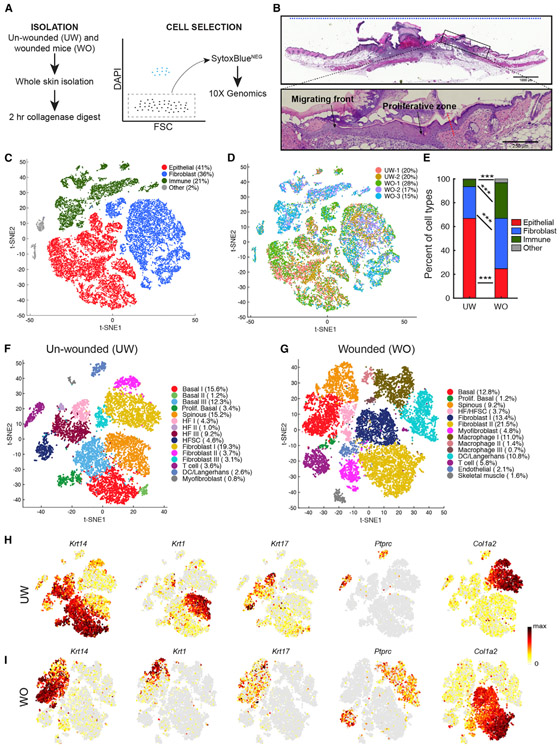
Figure 1.
scRNA-Seq Analysis of All Cells in the UW and WO Skin
(A) Schematic diagram detailing the single-cell isolation and live-cell selection strategy. (B) H&E analysis of WO skin showing a region equivalent to those used for scRNA-Seq. The blue dashed line at...
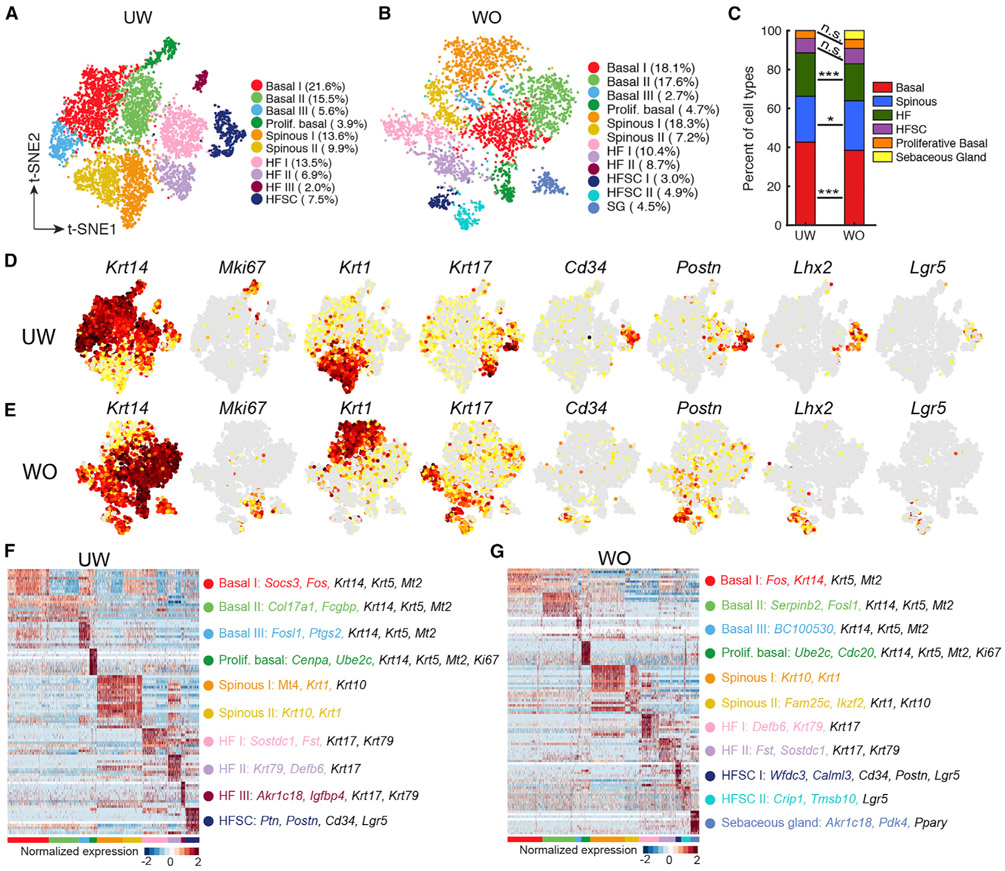
Figure 2.
scRNA-Seq Analysis Reveals Mild Changes in Epithelial Cellular Makeup during Wound Healing
(A) tSNE plot for all epithelial cells from UW skin with cell each type indicated. The percentage of cells in each cluster per total number (7,099) of cells under analysis is indicated in parenthesis....
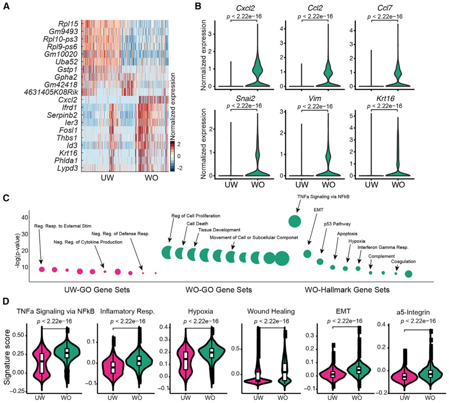
Figure 3.
Gene Expression Differences between Epidermal Basal Cells of the UW and WO Skin
(A) Heatmap showing the top 10 markers for basal cells from the UW and WO samples. All the identified markers are listed in Table S4 . (B) Expression of select genes in UW and WO basal cells. p values...
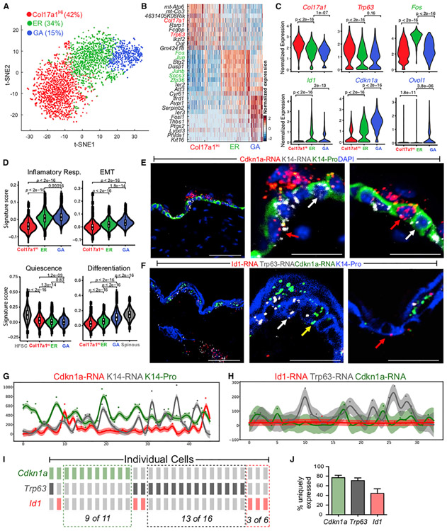
Figure 4.
scRNA-Seq and RNAScope Data Revealing Heterogeneity within UW Epidermal Basal Cells
(A) tSNE plot for NP basal cells from two UW replicates. The percentage of each subpopulation per total number (2,838) of basal cells was indicated. (B) Heatmap of top 10 markers for each subcluster i...
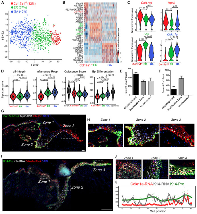
Figure 5.
Basal Cell Heterogeneity in WO Skin
(A) tSNE plot for NP basal cells from two WO replicates. WO-2 was not included in this analysis given its low basal cell number. The percentage of each subpopulation per total number (1,555) of basal ...
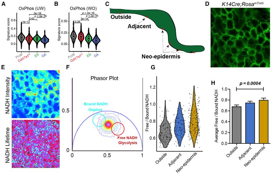
Figure 6.
FLIM Data Validating scRNA-Seq-Predicted Metabolic Heterogeneity in WO Skin
(A) Gene scoring analysis of all four UW basal subclusters using an oxidative phosphorylation signature. p values are from two-sided Wilcoxon rank-sum tests. (B) Gene scoring analysis of all four WO b...
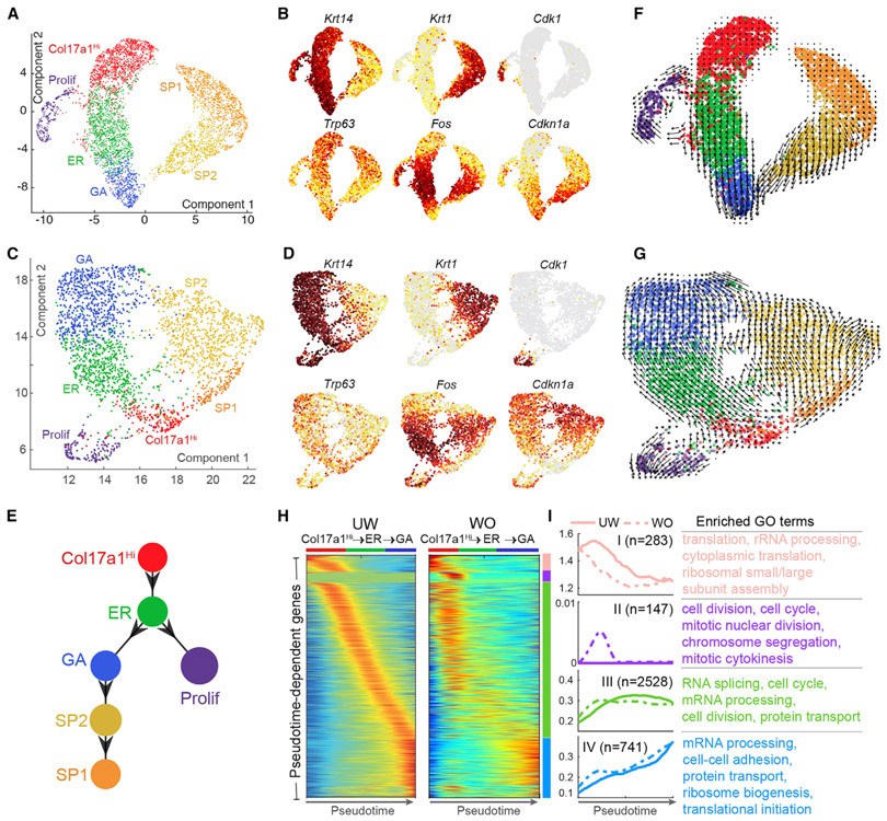
Figure 7.
Pseudotemporal Dynamics Analysis of Interfollicular Epidermal Cells in UW and WO Skin
(A) UMAP dimensional reduction of all UW epidermal cells. Cells are colored by the annotated identity. (B) Feature plots of (A) for the indicated genes. Cells are colored by the normalized expression,...
Figure images are served from the NIH/NLM PubMed Central Open Access Subset or Europe PMC; copyright remains with the publishers and authors.
💬 Discussion
0 commentsNo comments yet. Be the first to start a discussion!
Leave a Comment