Abstract
Abstract Calcium imaging is a powerful tool for recording from large populations of neurons in vivo. Imaging in rhesus macaque motor cortex can enable the discovery of fundamental principles of motor cortical function and can inform the design of next generation brain-computer interfaces (BCIs). Surface two-photon imaging, however, cannot presently access somatic calcium signals of neurons from all layers of macaque motor cortex due to photon scattering. Here, we demonstrate an implant and imaging system capable of chronic, motion-stabilized two-photon imaging of neuronal calcium signals from macaques engaged in a motor task. By imaging apical dendrites, we achieved optical access to large populations of deep and superficial cortical neurons across dorsal premotor (PMd) and gyral primary motor (M1) cortices. Dendritic signals from individual neurons displayed tuning for different directions of arm movement. Combining several technical advances, we developed an optical BCI (oBCI) driven by these dendritic signalswhich successfully decoded movement direction online. By fusing two-photon functional imaging with CLARITY volumetric imaging, we verified that many imaged dendrites which contributed to oBCI decoding originated from layer 5 output neurons, including a putative Betz cell. This approach establishes new opportunities for studying motor control and designing BCIs via two photon imaging.
🔬 Techniques
🔭 Microscopes
🧬 Organisms
✨ Fluorophores
🧪 Sample Preparation
🏭 Microscope Brands
🧪 Reagent Suppliers
🔎 Objectives
💻 Software Details
💻 Code & Software
Bus communication layer and data logger for Simulink Real Time (xPC Target)
cell detection in calcium imaging recordings
a visualization method for neural data
An implementation of demixed Principal Component Analysis (a supervised linear dimensionality reduction technique)
Code for real-time, low-latency processing of 2P calcium imaging data streaming from PrairieView
Tools for processing 2P recordings
Dear ImGui: Bloat-free Graphical User interface for C++ with minimal dependencies
💾 Data Repositories
🏛️ Research Organizations (ROR)
Affiliated research institutions:
📋 Methods
Animal subjects
All procedures and experiments were approved for animals S, W, and X by the Stanford University Institutional Animal Care and Use Committee (IACUC), and for animal L by the University of Texas at Austin IACUC and were performed in compliance with the Guide for the Care and Use of Laboratory Animals. Three male rhesus macaques (X, S, and W) were used for 2P imaging experiments and a fourth rhesus macaque (L) was used for secondary validation of virus constructs in V1. Stable 2P imaging during the reaching task was demonstrated in Subjects S, W, and X. Decode experiments were performed with subject X.
Subjects
S and W did not exhibit functionally tuned responses due to a lack of GCaMP expression (monkey S) or static non-modulated expression (monkey W). Monkey W did exhibit healthy GCaMP expression at some injection sites, but neurons in those sites were not responsive during the task (data not shown). All four animal subjects (S, W, X, and L) were included in the Neutralizing antibody assay results.
Assay for measuring AAV neutralizing antibodies
Individual subjects have different immunological states based on their particular exposure history to environmental viruses 124 . Although the brain has immune-privileged properties, whether pre-injection immunological status affects CNS expression of virally delivered constructs or elicits a systemic immune response is uncertain 52 . As such, viral infection and injection-related adaptive immune response may be highly variable between individuals, leading to consequences such as neutralization before infection, low expression of GCaMP, and/or deleterious systemic immune sensitization in certain subjects but not others. We employed a neutralizing antibody assay to quantify the levels of functionally neutralizing anti-AAV antibodies in serum samples. Our goal was to select specific serotypes of AAV with a higher probability to infect neurons and a lower probability of eliciting an immune response. As anticipated, each macaque subject had a different pre-existing antibody status; monkey S was responsive to AAV1, monkey W was responsive to AAV8, and monkey X to neither (Supplementary Fig. 3c ). After viral injection, we found that one monkey subject with significant pre-injection anti-AAVs (monkey W) developed significant antibody responses to AAV viruses injected into cortex (Supplementary Fig. 3d ). In contrast, a low anti-AAV monkey (monkey X) demonstrated a response profile that seemed to mimic a primary exposure (Supplementary Fig. 3e ), consistent with a previous report 125 . We caution that we do not have direct evidence that our particular serotype selection ensured better expression in our subject. While these results are consistent with our expectations, further experiments and additional subjects are required to validate the efficacy of this approach. In addition, the impact of immunoreactivity on the longevity of expression at healthy levels and on the success of subsequent additional injections remains to be determined. Blood samples were collected from four rhesus macaques. Blood draws were either performed at Stanford University (monkeys S, W, X) or at the University of Texas at Austin monkey (L), depending on the location of the monkey. Approximately 1 mL of blood was drawn at each collection date. Blood samples were placed in an IEC Centra GP8 Centrifuge at 1292× g (2500 RPM) for 150 s, transferred to a 1.5 mL Eppendorf, and then centrifuged at 22,131× g (14,000 RPM) for 3 min in an Eppendorf Centrifuge 5430. Remaining serum was extracted and stored at −80 °C until use. We compared neutralizing antibody titers in blood sera collected before and after intracranial injections of AAVs using a standard in vitro assay (see Supplementary Table. 1 ). HEK cells were seeded onto a clear bottom, black 96-well microplate (Corning Inc.) in dMEM/F12 without phenol red (Gibco Inc.) containing 10% Fetal Bovin Serum and incubated for 24 h at 37 °C with 5% CO 2 . The next day, serum dilutions were prepared (1:5, 1:25, 1:50, and 1:250), added to diluted adeno-associated virus encoding eYFP (AAV-Ef1α-eYFP), 1:1 volume-to-volume ratio, and for 1 h at 37 °C (see Supplementary Table 2 for AAV concentrations). Next, 10 μL of the serum-virus mixture was added to each well of cultured cells, resulting in final serum concentrations or 1:100, 1:500, 1:1000, and 1:5000. Experiments were run in triplicate for each condition. Positive control (no serum) and negative control (no AAV) wells were included in each experiment. For the pre-injection neutralization experiment, two serum dilutions were prepared (1:5 and 1:25), added to diluted adeno-associated virus encoding eYFP (AAV-Ef1α-eYFP), 1:1 volume-to-volume ratio, and for 1 h at 37 °C (see Supplementary Table 2 for AAV concentrations). Next, 10 μL of the serum-virus mixture was added to six wells of cultured cells. A positive, no serum, control was included for each serotype. Thirty-six or forty-eight hours after incubation, wells were imaged and YFP fluorescence measured. Fluorescence was quantified using a Tecan Infinite M1000 Microplate Reader. For each serum dilution, pre-injection and post-injection sera were compared using unpaired t-tests. In addition, widefield images of each well were captured using a Leica DMi8 microscope (10× objective) to visualize YFP expression. Cell lines were not authenticated.
Show full methods section
Animal subjects
All procedures and experiments were approved for animals S, W, and X by the Stanford University Institutional Animal Care and Use Committee (IACUC), and for animal L by the University of Texas at Austin IACUC and were performed in compliance with the Guide for the Care and Use of Laboratory Animals. Three male rhesus macaques (X, S, and W) were used for 2P imaging experiments and a fourth rhesus macaque (L) was used for secondary validation of virus constructs in V1. Stable 2P imaging during the reaching task was demonstrated in Subjects S, W, and X. Decode experiments were performed with subject X.
Subjects
S and W did not exhibit functionally tuned responses due to a lack of GCaMP expression (monkey S) or static non-modulated expression (monkey W). Monkey W did exhibit healthy GCaMP expression at some injection sites, but neurons in those sites were not responsive during the task (data not shown). All four animal subjects (S, W, X, and L) were included in the Neutralizing antibody assay results.
Assay for measuring AAV neutralizing antibodies
Individual subjects have different immunological states based on their particular exposure history to environmental viruses 124 . Although the brain has immune-privileged properties, whether pre-injection immunological status affects CNS expression of virally delivered constructs or elicits a systemic immune response is uncertain 52 . As such, viral infection and injection-related adaptive immune response may be highly variable between individuals, leading to consequences such as neutralization before infection, low expression of GCaMP, and/or deleterious systemic immune sensitization in certain subjects but not others. We employed a neutralizing antibody assay to quantify the levels of functionally neutralizing anti-AAV antibodies in serum samples. Our goal was to select specific serotypes of AAV with a higher probability to infect neurons and a lower probability of eliciting an immune response. As anticipated, each macaque subject had a different pre-existing antibody status; monkey S was responsive to AAV1, monkey W was responsive to AAV8, and monkey X to neither (Supplementary Fig. 3c ). After viral injection, we found that one monkey subject with significant pre-injection anti-AAVs (monkey W) developed significant antibody responses to AAV viruses injected into cortex (Supplementary Fig. 3d ). In contrast, a low anti-AAV monkey (monkey X) demonstrated a response profile that seemed to mimic a primary exposure (Supplementary Fig. 3e ), consistent with a previous report 125 . We caution that we do not have direct evidence that our particular serotype selection ensured better expression in our subject. While these results are consistent with our expectations, further experiments and additional subjects are required to validate the efficacy of this approach. In addition, the impact of immunoreactivity on the longevity of expression at healthy levels and on the success of subsequent additional injections remains to be determined. Blood samples were collected from four rhesus macaques. Blood draws were either performed at Stanford University (monkeys S, W, X) or at the University of Texas at Austin monkey (L), depending on the location of the monkey. Approximately 1 mL of blood was drawn at each collection date. Blood samples were placed in an IEC Centra GP8 Centrifuge at 1292× g (2500 RPM) for 150 s, transferred to a 1.5 mL Eppendorf, and then centrifuged at 22,131× g (14,000 RPM) for 3 min in an Eppendorf Centrifuge 5430. Remaining serum was extracted and stored at −80 °C until use. We compared neutralizing antibody titers in blood sera collected before and after intracranial injections of AAVs using a standard in vitro assay (see Supplementary Table. 1 ). HEK cells were seeded onto a clear bottom, black 96-well microplate (Corning Inc.) in dMEM/F12 without phenol red (Gibco Inc.) containing 10% Fetal Bovin Serum and incubated for 24 h at 37 °C with 5% CO 2 . The next day, serum dilutions were prepared (1:5, 1:25, 1:50, and 1:250), added to diluted adeno-associated virus encoding eYFP (AAV-Ef1α-eYFP), 1:1 volume-to-volume ratio, and for 1 h at 37 °C (see Supplementary Table 2 for AAV concentrations). Next, 10 μL of the serum-virus mixture was added to each well of cultured cells, resulting in final serum concentrations or 1:100, 1:500, 1:1000, and 1:5000. Experiments were run in triplicate for each condition. Positive control (no serum) and negative control (no AAV) wells were included in each experiment. For the pre-injection neutralization experiment, two serum dilutions were prepared (1:5 and 1:25), added to diluted adeno-associated virus encoding eYFP (AAV-Ef1α-eYFP), 1:1 volume-to-volume ratio, and for 1 h at 37 °C (see Supplementary Table 2 for AAV concentrations). Next, 10 μL of the serum-virus mixture was added to six wells of cultured cells. A positive, no serum, control was included for each serotype. Thirty-six or forty-eight hours after incubation, wells were imaged and YFP fluorescence measured. Fluorescence was quantified using a Tecan Infinite M1000 Microplate Reader. For each serum dilution, pre-injection and post-injection sera were compared using unpaired t-tests. In addition, widefield images of each well were captured using a Leica DMi8 microscope (10× objective) to visualize YFP expression. Cell lines were not authenticated.
Surgical procedures
In monkey X, we implanted the imaging chamber in a sequence of two surgeries in order to (1) minimize the duration of surgical procedures, and (2) allow for behavioral training with head fixation prior to opening the dura. After the dura was opened, the surface of the cortex required intermittent cleaning and maintenance, and an opaque neomembrane often began to grow over the surface of the cortex approximately 2–4 months after opening the dura. In the first surgery, we implanted the chamber over the surface of the bone, sealing the chamber to bone interface with C&B Metabond dental cement (Parkell), and cementing the chamber in place using Palacose bone cement (Heraeus Medical) and titanium bone screws (Synthes Inc.). Custom-machined headposts were implanted to allow for head fixation during behavioral training. Several months later, after completing behavioral training, we performed a second surgery to remove the skull (in the region of the cylinder) and dura from the center of the 2P chamber, to perform viral injections and to place the artificial dura (AD). Viral constructs were injected using pulled glass micropipettes (~25 μm tips), beveled using a micropipette grinder (Narishige EG-401 pipette beveller) using a nanoliter injector (WPI Inc.). To assist in visualizing viral injections, trypan blue dye (0.4% (w/v)) was diluted 1:10 in saline and mixed with the viral suspension 21 . For monkeys S and W, we implanted an earlier generation of titanium chamber design, which threads into a craniotomy. For these surgeries, the imaging chamber was implanted in a first surgery, but the dura was left intact, and virus injections were performed using stainless steel syringes (Hamilton) outside the operating room while the monkey was performing a behavioral task. After waiting for expression, the dura was then resected, and the AD placed in a second surgery. While this approach has the advantage of not exposing the surface of the brain while waiting for GCaMP expression (~8 weeks) prior to imaging, it required injections to be performed through the dura, preventing careful targeting of virus as the vasculature on the surface of cortex was not visible. This led to additional uncertainty with regards to injection location and depth, made it impossible to avoid surface vasculature while injecting, and increased the required volume of virus injected in order to be confident that a sufficient volume of virus was injected in the target lamina. As such, in monkey X we adopted the more targeted approach, performing virus injections using glass micropipettes with the surface of the brain exposed, which is the preferred approach for future experiments 21 .
Implant design and maintenance
The imaging chamber design strikes a balance between (1) enabling imaging access to a large volume of tissue (18 mm visible, of which a 12 mm diameter region is accessible for 2P imaging down to ~1000 µm deep using the Nikon 16 × 0.8 NA lens) using commercially available multiphoton objective lenses and (2) minimizing the implant size. The implant must allow for stable head fixation during reaching behaviors, and allow for simple replacement of the silicone AD and access to the edge of the dura for routine cleaning and maintenance. These design constraints suggest a large diameter but low-profile imaging chamber and multi-point head fixation. Design files for the chamber and associated hardware are provided in supplemental materials. After an experiment, the tissue stabilizer was removed, and a solution of agarose and vancomycin was applied to the dura edge, typically every 1–4 days. Physiosol (Pfizer Inc.) with added vancomycin was applied to fill the remaining chamber volume, and the glass window was secured in place with the retainer ring, and the chamber cap is secured on top. Under normal conditions, the AD did not need to be regularly removed or replaced for cleaning. Over timescales of several months, we observed “neomembrane” tissue growth under the AD but over the surface of the cortex. Over time, this tissue grew in thickness, blocking optical access to the cortex, and requiring careful surgical dissection and removal. In practice, the timeline for tissue removal could be variable but was usually required every 2–4 months to retain imaging performance. The wound margin at the edge of the durotomy also experienced tissue growth and required periodic trimming to prevent excessive buildup of tissue above the artificial dura. Head restraint and implant immobilization Initial testing revealed that single-point head fixation methods, as are commonly used for electrophysiology, were incapable of restricting tissue motion at the scale of microns. We tested a three-point acrylic-free footed headpost system that uses bone screws to secure headposts to the skull, and found that this too was not sufficient to restrict micron-scale implant motion during arm-movement behavior. Instead, we found that using a single larger implant constructed with bone cement (Palacose, Zimmer BIOMET Inc.) and titanium mandible straps (Synthes Inc.) fixed to the skull with bone screws allowed for more rigid fixation by distributing the loads between the multiple fixation points through the bone cement. Design files for the head restraint and associated hardware are provided in supplemental materials and details provided upon reasonable request. Tissue stabilization Prior to imaging, the outer window and retaining ring were removed under sterile conditions, and the AD was exposed to the air. The tissue stabilizer was placed within the chamber, placing gentle mechanical pressure on the top surface of the AD. The tissue stabilizer consisted of a conical aluminum component which sat inside the chamber and held a circular glass coverslip against the artificial dura. Since the location of the surface of the brain could change over time due to tissue growth, recession, or other factors, we fabricated a set of tissue stabilizers at different fixed depths in 500 µm increments. Sterile saline was placed in the chamber prior to placing the stabilizer as an index matching fluid between the silicone and stabilizer glass. Widefield Imaging in V1 As part of the development and verification process for the GCaMP constructs, we validated some constructs using widefield imaging in visual cortical areas in monkey L (Supplementary Fig. 5 ). We used a large (6 × 6 deg 2 ) sine wave grating at 100% contrast with a spatial frequency of 2 cpd. The mean luminance of the screen was set at 30 cd/m 2 .The grating was flashed with a temporal frequency of 4 Hz (100 ms on, 150 ms off), while the monkey was performing a fixation task. The behavioral task and widefield (1P) GCaMP data analysis in the rhesus macaque (monkey L) were performed as described previously 21 .
Two-photon imaging in premotor primary motor
(M1) cortex Imaging was performed using a Bruker Ultima in vivo microscope with a custom motorized orbital nosepiece (Bruker Inc.) to provide off-axis imaging with a Nikon 16 × 0.8 NA objective lens. Images were acquired at 512 × 512 resolution at a single depth at 30.3 Hz using resonant-scanning galvanometers (or occasionally at lower resolution and higher framerate, while imaging a portion of the 512 × 512 pixel field). Laser power was adjusted as necessary to optimize SNR prior to each recording series and typical values were between 50–150 mW. Using dichroic beam splitter (555 nm) and a pair of filters, we collected both a functional green channel (520/44 nm) and a static red fluorescent channel (624/40 nm) to facilitate registration. Typical sessions in which the subject was working in the imaging rig lasted between 90–180 min. Imaging was performed during decode blocks, typically lasting between 5–30 min, and different decoding sessions were performed in different fields of view during a single session in order to explore different injection sites and depths. We typically performed imaging (while the monkey was at rest and not performing the task) for several minutes in between decode blocks to localize distinct fields of view with neural features, or to localize an imaging field of view based on the surface vasculature. We did not observe photobleaching over the course of a decode block or across blocks within a session in the same region. 2P imaging sessions were collected over sessions spanning the following number of days in the three subjects included here: monkey S, 122 days; monkey W, 30 days; monkey X, 144 days. We note that for all three subjects, degradation of imaging quality was not a driver for terminating experiments, and imaging data were collected until we had sufficient data within the imageable injection regions. In particular, for monkey W, imaging quality remained excellent but as we did not observe functional tuning in the neurons we imaged, we did not continue to collect data beyond the first month of exploration after observing virus expression. The positioning of the imaging plane for each decode session was chosen to maximize the number of modulated processes observed in the field of view. We did not attempt to optimize correspondence of the imaging field of view across sessions. Behavioral task Monkey X was trained to make point-to-point reaches with the arm contralateral to imaging implant on a delayed center-out-and-back task in a vertically-oriented 2D plane as described previously 126 . The monkey initiated each trial by holding a point at the center of a display screen, placed approximately 30 cm from the eyes. Next, one of four radially arranged targets appeared 10 cm from the center and jittered around the target location (5–10 mm std. deviation) during the delay period (randomized period, ranging from 100 to 700 ms). Next the target ceased to jitter, and the central fixation point disappeared, thereby indicating a “go cue”. The monkey was free to initiate a reach following the “go cue”. Movement onset was defined as the time when in-plane hand speed exceeded 5% of peak speed for each trial. We note that movement onset is defined entirely behaviorally, independently of neural responses. Reaction time (RT) was defined as the time between the “go cue” and movement onset. To exclude rare trials where the monkey may have anticipated the “go cue” (i.e., RTs < 180 ms) or where the monkey may have been distracted (i.e., RTs > 620 ms), we aborted trials in real time by blanking the screen and withholding reward if the RT was outside of the 180–620 ms RT range. Hand position was measured in 3D and in real time with a Polaris infrared bead tracker (Polaris, Northern Digital, Ontario, Canada) which samples 60 times/s with submillimeter accuracy. Liquid rewards were delivered automatically upon successful target acquisition and hold in the delayed-reach task, or upon successful target decode in the oBCI task, which operated in the same way but rendered a magenta annulus around the decoded target upon successful decode, or gray for unsuccessful decode. Task timing, stimulus control, and behavior monitoring were performed using Simulink with real-time xPC target (Mathworks Inc., Natick, MA) while microscope control, image acquisition, and online decode were performed by a separate PC (Fig. 6a ). Behavioral and task data were serialized and sent via UDP to a data logging PC running custom data logging software available online ( https://github.com/djoshea/matudp ). Images were acquired continually throughout the duration of the task (not triggered on individual trials) using PrairieView software (Bruker Instruments, Inc.). Offline ROI identification and analysis of neuronal responses We processed each imaging session offline using Suite2P 53 ( https://github.com/MouseLand/suite2p ) and analyzed 36 imaging decode sessions collected on 8 days. Imaging datasets were aligned using the red, static fluorescence channel using a rigid coarse alignment step followed by a non-rigid block-wise alignment step. Standard settings for the algorithm were used with the following exceptions to optimize for dendritic ROIs and GCaMP6f (connected = False, tau = 0.7). We identified putative dendritic/axonal ROIs in the datasets as those ROIs with a computed aspect ratio greater than 2 (ratio of long axis to short axis of ROI shape), and manually verified that this selection criterion identified only ROIs that appeared to be neuronal processes. We next performed a clustering analysis on individual functional ROI responses to check whether automatic ROI detection approach identified distinct neuronal signals rather than signals from a small set of individual neurons split into many separate ROIs. First, we assembled for each ROI a vector of trial-averaged responses aligned to movement onset for each reaching direction. These response vectors were then clustered using DBSCAN, a non-parametric density-based clustering algorithm. DBSCAN which looks for clusters of points (ROIs), which are packed more closely together in feature space (have highly similar response profiles during reaching). DBSCAN can automatically determine the number of clusters present in the data. For all 36 datasets, DBSCAN identified only a single cluster including the vast majority of ROI responses, excluding a small fraction of ROIs, containing noise, that were highly dissimilar to all of the other ROIs and to each other. This indicates that in our imaging datasets, ROI responses form a continuum in the space of peri-movement responses, rather than distinct, separable clusters. The latter would be expected if the signals originated from the extended arbors of a small number of neurons. We also directly verified this non-clustered continuum in response space by using a t-SNE visualization (Supplementary Fig. 8d, e ). We next performed a pairwise correlation analysis to identify pairs of putative dendritic/axonal ROIs which likely originate from the same neuron following the method described in ref. 30 . At the threshold of ρ ≥ 0.8, 187/4365 ROIs were identified as likely recorded from the same neuron as another ROI in the datasets. At a more conservative threshold of ρ ≥ 0.6, 828/4365 possible duplicates were detected. All dendritic ROIs were retained for subsequent analysis. Enhanced mean images were computed by averaging all frames of the registered data tensor, and then computing the inverse hyperbolic sine of the value of each pixel to enhance contrast (only for visualization). Δ F / F 0 was estimated from extracted fluorescence traces using an iterative time-varying baseline estimate following Peters et al. (2014) 115 . Single trial rasters were visualized by sorting ROIs using rastermap ( https://github.com/MouseLand/rastermap ), an embedding algorithm which groups similar ROIs nearby to reveal structure in the traces. Z -scored responses were computed relative to the mean and standard deviation of fluorescence levels observed during a pre-trial baseline period when the hand was stationary. To assess individual ROI’s responsiveness to task events, we extracted on each trial, the fluorescence level of each ROI within a time window just prior to the task event and immediately following the task event, and compared the distributions across trials using a rank-sum test. For the target cue and go cue, we compared frames within the window of −150 to 0 ms prior with frames in the window 0–150 ms after. For movement onset, we compared 450–100 ms prior with 0–350 ms after, as neural responses accompanying movement typically begin in advance of movement persist throughout the reach. We computed the onset time of directionally-tuned responses in each ROI by performing a Kruskal–Wallis nonparametric one-way analysis of variance on the single-trial fluorescence measurements at each time in a sliding window. The onset time is taken when significance at p < 0.01 is reached for five consecutive 10 ms windows. Direction-tuning was assessed by collecting the single trial average fluorescence levels of each ROI in the 350 ms following movement onset, and grouping these values by reach direction condition. ROIs were considered direction-tuned if an ANOVA test for a main effect of reach-direction significantly affected the mean fluorescence level at p < 0.01. For these tuned ROIs, we then constructed a tuning map by regressing each ROI’s activity onto 2D hand velocity using an empirically determined 50 ms lag between neural activity and hand velocity (neural leads kinematics). We converted these coefficients into a preferred direction angle, which we mapped into a perceptually uniform circular colormap (CET-C2, Peter Kovesi, https://peterkovesi.com/projects/colourmaps/ ). Colored ROI masks then were then painted onto the mean image using a transparency map derived from the product of the strength of the directional tuning of the entire ROI and the ROI mask weights onto pixels. To visualize neural trajectories, we first computed the trial-averaged z -scored ROI responses for all direction-tuned ROIs in a window 300 ms before to 400 ms after movement onset. We used demixed PCA ( https://github.com/machenslab/dPCA ) to identify a condition-independent signal (CIS) dimension exhibiting variance over time but with minimal cross-condition variance (corresponding to reach direction). For DPCA, the lambda hyperparameter was determined automatically for each session using cross-validation. To identify a subspace of dimensions exhibiting variance related to X and Y reach direction, we used targeted dimensionality reduction (TDR) 55 . Essentially, we compute the pseudoinverse of the matrix of X and Y velocity regression coefficients for each direction-tuned ROI to obtain these dimensions. We then successively orthonormalize the CIS, TDR X, and TDR Y dimensions. Trial-averaged and single trial ROI trajectories are then projected into these dimensions for visualization. To assess the stability of tuning individual ROIs within imaging sessions, we separately assessed preferred directions for each ROI for the first 25% and last 25% of each session. We computed the difference of preferred directions and a null distribution computed as the difference of preferred directions computed from 1000 random reshufflings of these early/late imaging frame labels. Drifts of preferred directions was considered significant if the absolute change in preferred direction exceeded that of 99% of the random shuffles ( p < 0.01). To assess the heterogeneity of tuning within individual ROIs, we regressed each individual pixel within an ROI onto hand velocity, producing a set of pixel-wise regression coefficients. We then performed K-means clustering on these coefficients and identified the optimal cluster count which maximized the Calinski-Harabasz criterion values. We considered an ROI to have multiple meaningful clusters if the optimal cluster count was greater than 1, and if at least 30% of the pixels belonged to at least two such clusters, and the difference in preferred direction corresponding to the centroid of these clusters were at least 60 degrees. Real-time oBCI decoding During oBCI decoding sessions (36 decode sessions collected on eight days), image data were accessed using PrairieLink (Bruker Instruments, Inc.), processed using a soft real-time C++/Cython/NumPy pipeline, which aggressively avoids memory copies to reduce latency. The code for this real-time decoding pipeline is documented and available at https://github.com/djoshea/obci/ . Frames were ignored until a fixed period of time after the go cue ( T skip ), after which frames are integrated for a fixed duration ( T int ) (Fig. 6b and Supplementary Fig. 14 ). T skip was selected to roughly match the average reaction time of the subject to begin movement, so as to avoid acquiring (for decode purposes) neural activity that is unlikely to be related to the reach target. Then, starting right after T skip , we acquired peri-movement neural activity during T int . This decoding nomenclature was used in a prior study from our group 8 . While it is possible to develop a mathematically optimal procedure for selecting T skip and T int , in practice, we found that it was helpful to use a permissive integration window to capture the natural behavioral variability of an animal, while also minimizing the number of non-informative imaging frames that contribute to the average frame calculation. We experimented with a range of values to improve decode performance and speed (Supplementary Fig. 14 ): T skip values ranged from 200 to 400 ms and T int values ranged from 70 to 200 ms. These ranges were selected based on several factors, including: Variability in the reaction time of the animal. The integration time should be centered around the beginning of the attempted movement. On trials in which an animal had a slow reaction time, the integration window could occur too early, before a decodable signal was present (in our data). As such, there exists a tradeoff between decoder speed and accuracy, taking behavioral variability into account. The typical timing of divergence of calcium signals within the imaging region, based on offline analysis, as shown in Fig. 6h, i . We note that this timing may be specific to the recording location and subpopulation of cells recorded. Image acquisition time (33 ms). Only full frames are considered during decode, so values of T int and T skip in practice are discretized by the frame period. Rather than create a multi-objective cost function to optimize these values, in practice, we chose to bias towards increased robustness by using a permissive Tint (long window) and short T skip to increase the likelihood of movement onset and peri-movement neural activity falling within the integration window. Each imaging frame was processed by applying an approximate Gaussian spatial blur (standard deviation of between 3 pixels) and accumulated into a running average (Fig. 6c ). During training trials, after T int , the average image was accumulated into the running average for the current target, Y i,j,k , where k ∈ 1, 2, 3, 4 indexes target location, and i , j index pixel [ x , y ] location. During decode trials, after T int , the reach target was decoded using a pixel-wise minimum mean square error (MMSE) decoder as described in Eq. ( 1 ): 1 documentclass[12pt]{minimal} usepackage{amsmath} usepackage{wasysym} usepackage{amsfonts} usepackage{amssymb} usepackage{amsbsy} usepackage{mathrsfs} usepackage{upgreek} setlength{oddsidemargin}{-69pt} begin{document}$$mathop{{rm{argmin}}}limits_{k}mathop{sum}limits_{{rm{i,j}}}{left({X}_{{rm{i,j}}}-{Y}_{{rm{i,j,k}}}right)}^{{bf{2}}},$$end{document} argmin k ∑ i,j X i,j − Y i,j,k 2 , X is the image formed by averaging frames acquired during the T int on the current trial. oBCI experimental sessions were often terminated to explore different imaging depths or fields of view the same day, as opposed to ending a session after observing roll-off of decode performance. In many if not most cases, we anticipate that the image decoder would continue to operate successfully for much longer than the acquired series of data. For online decode experiments, we sought to ensure that motion artifacts were not responsible for driving tuning and decode via several approaches: In post-hoc analysis of the data obtained during online decode experiments, we did not observe characteristic patterns of symmetric signal increase/decrease for opposite movements that we might expect if fluorescence modulation were primarily resulting from motion. In virtually every field of view imaged, only a sparse subset of neural features exhibited tuning, while the other fluorescent objects with a similar morphology did not. It would be quite unlikely, if not impossible, to obtain this result if the observed tuning were the result of motion artifacts. We performed online control experiments, imaging in areas with autofluorescence but no GCaMP expression and did not decode at above chance levels. For online decode experiments, we lightly blurred the images with gaussian smoothing to minimize the impact of X / Y translational movement. While Z -axis motion is not directly observable, during initial experimental characterization, we imaged dendrites during behavior at several focal planes, offset in depth in sequences of 5–10 µm. In all cases, we observed consistent tuning regardless of imaging plane position, further indicating that the observed tuning was not the result of z -axis motion artifact (data not shown). We minimized the impact of background light via several methods: The monkey and apparatus were in the dark throughout experimental sessions, with the only source of light being the illumination of targets displayed on the screen. Targets were either red or blue (not green) to minimize the likelihood of interfering with GCaMP signals, and LEDs or light sources were taped over. The geometry of the tissue stabilizer naturally blocks most residual background light due to the small space between the lens and the wall of the tissue stabilizer. If background light was ever found to be an issue, we placed blacked foil around the implant and objective. In practice, we found that background light did not present a major challenge during the course of these experiments. Offline analysis of decoder performance Offline classification was performed using scikit-learn 127 to implement multiclass support vector machine classification with 5-fold cross validation. Trials were filtered for successful reaches and aligned to either go cue or movement onset for separate analyses. Images were processed to calculate Δ F / F and integrated using a causal sliding 200 ms window, and all frames within this window were averaged prior to inclusion and preprocessed by removing the mean and scaling to unit variance for each feature (pixel). Imaging data was registered using NoRMCorre 128 prior to analysis. Offline analysis was performed using custom MATLAB (Mathworks Inc, Natick, MA) and Python code, available upon reasonable request. For the eigenvalue screen plots presented in Supplementary Fig. 12 , eigenvalues were calculated by running PCA on a 2d matrix formed by concatenating trials and time points along dimension 1, and unraveling all pixels from single frames along the second dimension. The final matrix has dimensions (# trials * # timepoints) x (# xPixels * # yPixels). The offline pixel dropping analysis presented in Supplementary Fig. 15 was performed by selecting 15 square regions of a given size, sampled at random from the full field of view and masking all pixels outside of that square. The masked data was then decoded using the same approach described above for multiclass classification.
CLARITY tissue clearing and imaging
The area of interest was dissected from the whole brain and embedded in 1% hydrogel. The tissue was cleared in the SmartClear (Lifecanvas Inc.) for 2 weeks, then stained with anti-GFP conjugated to alexa-647 (Invitrogen Inc.) and lectin conjugated to DyLight 488 (antibody concentrations 1:100 in PBST with 1% triton-x and 0.2% sodium azide) for 1 week, and finally washed in PBST for 1 week prior to imaging. The tissue was immersed in RapiClear (SunJin Lab Co) for 2 days and then imaged using an Olympus two-photon microscope with 10 × 0.6 NA CLARITY objective.
Open-source software
We thank the authors and contributors of the following open-source projects utilized in this project: Cython— https://cython.org/ Numba— http://numba.pydata.org/ SciPy 130 /NumPy/Matplotlib— https://www.scipy.org/ https://numpy.org/ https://matplotlib.org/ Jupyter— https://jupyter.org/ Sci-kit learn 127 — https://scikit-learn.org/ Suite2P 53 — https://github.com/cortex-lab/Suite2P Rastermap— https://github.com/MouseLand/rastermap dPCA 54 — https://github.com/machenslab/dPCA CET Perceptually Uniform Color Maps 131 — https://peterkovesi.com/projects/colourmaps/ Libuv— http://libuv.org/ Dear ImGui— https://github.com/ocornut/imgui Cygwin— https://www.cygwin.com/ Reporting summary Further information on research design is available in the Nature Research Reporting Summary linked to this article.
Surgical procedures
In monkey X, we implanted the imaging chamber in a sequence of two surgeries in order to (1) minimize the duration of surgical procedures, and (2) allow for behavioral training with head fixation prior to opening the dura. After the dura was opened, the surface of the cortex required intermittent cleaning and maintenance, and an opaque neomembrane often began to grow over the surface of the cortex approximately 2–4 months after opening the dura. In the first surgery, we implanted the chamber over the surface of the bone, sealing the chamber to bone interface with C&B Metabond dental cement (Parkell), and cementing the chamber in place using Palacose bone cement (Heraeus Medical) and titanium bone screws (Synthes Inc.). Custom-machined headposts were implanted to allow for head fixation during behavioral training. Several months later, after completing behavioral training, we performed a second surgery to remove the skull (in the region of the cylinder) and dura from the center of the 2P chamber, to perform viral injections and to place the artificial dura (AD). Viral constructs were injected using pulled glass micropipettes (~25 μm tips), beveled using a micropipette grinder (Narishige EG-401 pipette beveller) using a nanoliter injector (WPI Inc.). To assist in visualizing viral injections, trypan blue dye (0.4% (w/v)) was diluted 1:10 in saline and mixed with the viral suspension 21 . For monkeys S and W, we implanted an earlier generation of titanium chamber design, which threads into a craniotomy. For these surgeries, the imaging chamber was implanted in a first surgery, but the dura was left intact, and virus injections were performed using stainless steel syringes (Hamilton) outside the operating room while the monkey was performing a behavioral task. After waiting for expression, the dura was then resected, and the AD placed in a second surgery. While this approach has the advantage of not exposing the surface of the brain while waiting for GCaMP expression (~8 weeks) prior to imaging, it required injections to be performed through the dura, preventing careful targeting of virus as the vasculature on the surface of cortex was not visible. This led to additional uncertainty with regards to injection location and depth, made it impossible to avoid surface vasculature while injecting, and increased the required volume of virus injected in order to be confident that a sufficient volume of virus was injected in the target lamina. As such, in monkey X we adopted the more targeted approach, performing virus injections using glass micropipettes with the surface of the brain exposed, which is the preferred approach for future experiments 21 .
Supplementary information Supplementary Information Peer Review File Description of Additional Supplementary Files Supplementary Movie 1 - Example dendrite imaging Supplementary Movie 2 - real-time decode of reach behavior using 2P imaging Supplementary Movie 3 - CLARITY imaging of tissue volume Supplementary Data 1 Reporting Summary
📊 Figures
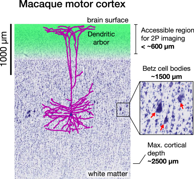
Fig. 1
Dendritic calcium signals are readily accessible from layer five neurons.
Two photon (2P) calcium imaging is currently capable of recording neural activity from the surface down to approximately 600u2009u00b5m (green region), but photon scattering poses a challenge for imag...
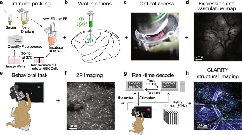
Fig. 2
Experimental pipeline for combining functional imaging during motor behaviors with structural imaging in macaque monkeys.
a Prior to imaging, we performed a neutralizing antibody assay in order to select an appropriate viral serotype tailored to the immune response of each monkey. b Viral constructs were injected into co...
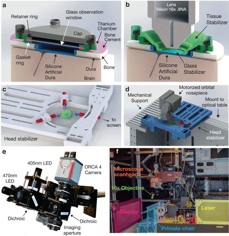
Fig. 3
Implantable chamber and imaging apparatus.
a Implantable titanium chamber in non-imaging configuration enabled observation through a glass window if the cap is removed. The glass window enabled long-term application of antibiotics and drugs to...
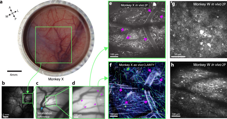
Fig. 4
Multiscale, multi-modal imaging.
a Imaging chamber with stabilizer in place under ambient illumination, approximately two weeks after implant. b Cortical surface imaged using widefield (1P) imaging (representative example expression ...
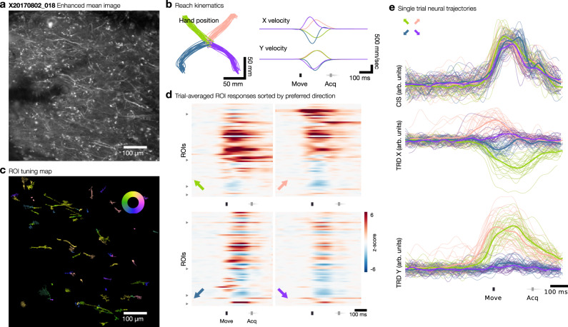
Fig. 5
Functional responses during reaching behavior.
a Contrast enhanced mean image of example FOV from Monkey X, site 2, one of 36 analyzed imaging sessions. b Reaching kinematics observed during behavioral task. Move indicates movement onset; Acq indi...
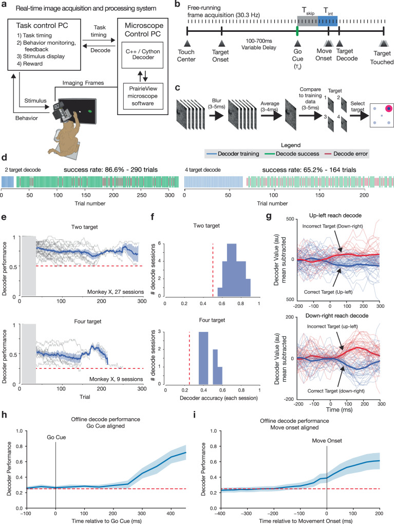
Fig. 6
Real-time decode of neural activity from functional imaging in motor cortex.
a Real-time stimulus control was implemented by decoding frames acquired from the microscope directly from memory buffers on the acquisition hardware. This provided rapid low-level access to imaging d...
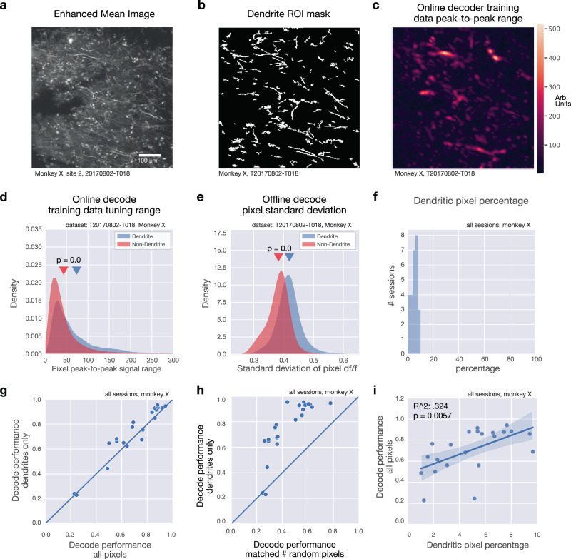
Fig. 7
Dendritic signals drive online decode.
a Mean intensity projection (contrast enhanced) for example imaging session (one of 36 sessions shown), b Dendrite ROI pixel mask for example in a . c Peak-to-peak pixel signal range across four reach...
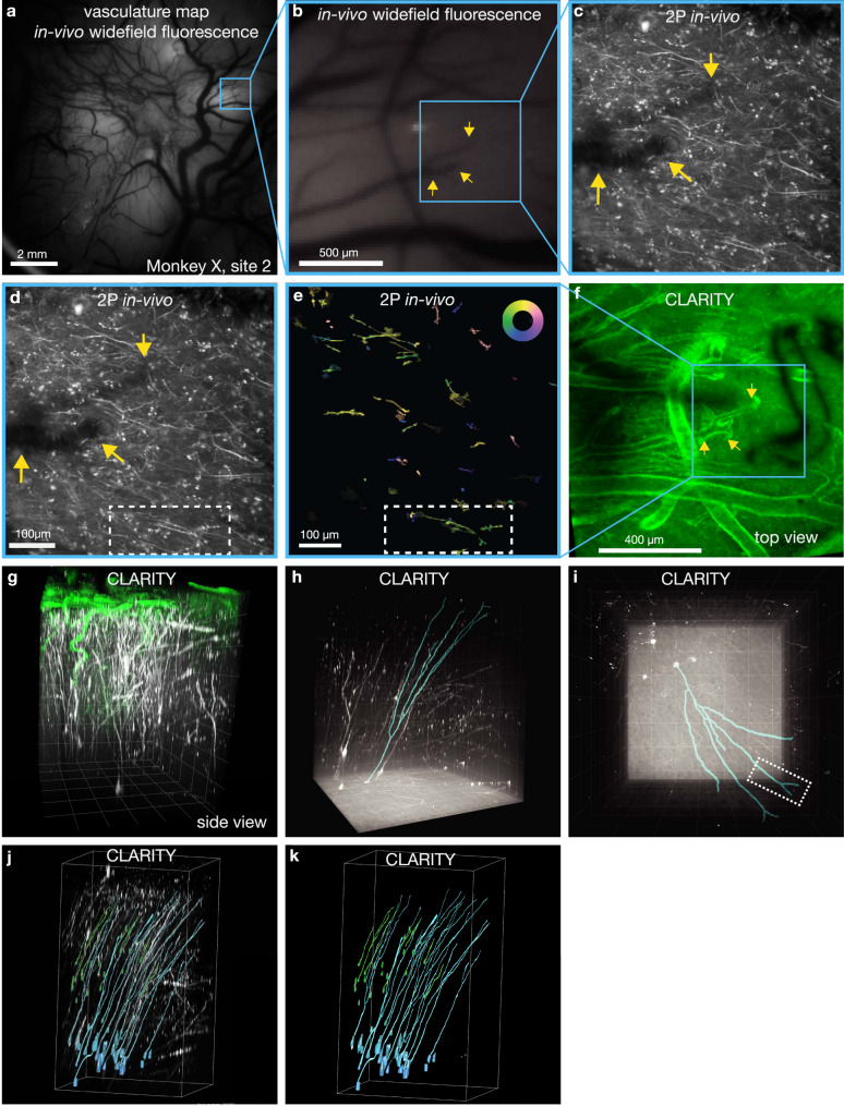
Fig. 8
Identifying neurons in CLARITY and functional imaging.
a A widefield fluorescence image revealing vasculature landmarks was used to locate and register 2P imaging FOVs (representative example widefield image from the start of each imaging session). b High...
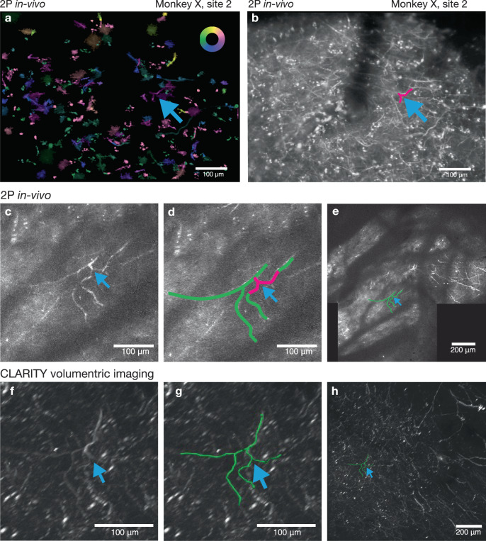
Fig. 9
A second example of a neural process functionally imaged and reconstructed in the registered CLARITY volume.
a Pixel-wise tuning map, same FOV and presentation style as in Fig. 4h (Inset color wheel indicates reach direction). A neural feature of interest is indicated by the blue arrow. b . Mean intensity pr...
Figure images are served from the NIH/NLM PubMed Central Open Access Subset or Europe PMC; copyright remains with the publishers and authors.
💬 Discussion
0 commentsNo comments yet. Be the first to start a discussion!
Leave a Comment