Abstract
Imaging neuronal networks provides a foundation for understanding the nervous system, but resolving dense nanometer-scale structures over large volumes remains challenging for light microscopy (LM) and electron microscopy (EM). Here we show that X-ray holographic nano-tomography (XNH) can image millimeter-scale volumes with sub-100-nm resolution, enabling reconstruction of dense wiring in Drosophila melanogaster and mouse nervous tissue. We performed correlative XNH and EM to reconstruct hundreds of cortical pyramidal cells and show that more superficial cells receive stronger synaptic inhibition on their apical dendrites. By combining multiple XNH scans, we imaged an adult Drosophila leg with sufficient resolution to comprehensively catalog mechanosensory neurons and trace individual motor axons from muscles to the central nervous system. To accelerate neuronal reconstructions, we trained a convolutional neural network to automatically segment neurons from XNH volumes. Thus, XNH bridges a key gap between LM and EM, providing a new avenue for neural circuit discovery.
🔬 Techniques
🧬 Organisms
💻 Software
✨ Fluorophores
🧪 Sample Preparation
🏭 Microscope Brands
📷 Detectors
💻 Software Details
💻 Code & Software
💾 Data Repositories
🏛️ Research Organizations (ROR)
Affiliated research institutions:
📋 Methods
Experimental Animals
Experimental procedures were approved by the Harvard Medical School Institutional Animal Care and Use Committee and performed in accordance with the Guide for Animal Care and Use of Laboratory Animals and the animal welfare guidelines of the National Institutes of Health.
Mice
(Mus musculus) used in this study were C57BL/6J-Tg(Thy1-GCaMP6s)GP4.3Dkim/J, male, 32 weeks and C57BL/6, male, 28 weeks, ordered through Jackson Laboratory (The Jackson Laboratory, Bar Harbor, ME). Mice were housed up to 4 per home cage at normal temperature and humidity on reverse light cycle, and relocated to clean cages every two weeks. Flies ( Drosophila melanogaster ) used in this study were 1–7 day old female adults with the w1118 genetic background. The transgenic approach for labeling GABAergic nuclei (used in Fig. 3 and Extended Data Fig. 5 ) is described below. See Life Sciences Reporting Summary for more details.
Sample preparation
Tissue samples were prepared for XNH imaging using protocols for electron microscopy (EM), including fixation, heavy metal staining, dehydration, and resin embedding 4 , 51 . For heavy metal staining, we used an enhanced rOTO protocol 51 for all mouse samples and some of the fly samples. For other fly samples, we modified the protocol to increase 4 or decrease heavy metal staining, but these variations did not have a large effect on XNH image quality. Following staining, samples were dehydrated in a graded ethanol series and embedded in either TAAB Epon 812 (Canemco) or LX112 (Ladd Research Industries) resin. Resin-embedded samples were polymerized at 60ºC for 2–4 days. Polymerized samples were trimmed down to a narrow (1 to 2 mm diameter) rod using either an ultramicrotome or a fine saw, then glued to an aluminum pin. To smooth rough surfaces on the samples, which introduce noise into the XNH images, mounted samples were covered in a small droplet of resin, and the droplet was polymerized at 60ºC for 2–4 days. For labeling APEX2-expressing cells (see below), we performed 3,3’-diaminobenzidine (DAB) staining after fixation and before heavy metal staining. Briefly, the nervous system from an adult female was dissected, fixed (2% glutaraldehyde, 2% formaldehyde solution in 100mM sodium cacodylate buffer with 0.04% CaCl2) at room temperature for 75 minutes then moved to 4ºC for overnight fixation in the same solution. The following day, the sample was washed in cacodylate buffer, then 50mM glycine in cacodylate buffer, then cacodylate buffer again. To stain APEX2-expressing cells, the sample was incubated with 0.03% DAB in cacodylate buffer for 30 minutes, then H 2 O 2 was added directly to the incubating samples to reach an H 2 O 2 concentration of 0.003% 52 . The reaction was allowed to continue for 30 minutes, after which the sample was washed in cacodylate buffer and inspected for visible staining product. Clusters of small brown puncta corresponding to the labeled nuclei were faintly visible ( Extended Data Fig. 1g , top panel). The DAB and H 2 O 2 incubations were repeated once more to increase the staining intensity. The sample was subsequently stained with 3-amino-1,2,4-triazole-reduced osmium 4 and uranyl acetate, then dehydrated and embedded in LX112 resin. We found that heavy-metal staining, typical for EM studies 51 , improves membrane contrast in XNH images. However, heavy-metal staining also increases X-ray absorption, causing heating and warping of the sample and thereby degrading image resolution. To counteract sample warping, we imaged in cryogenic conditions and optimized X-ray dosage to maximize signal but avoid excessive heating 53 . Samples that had major alignment artifacts due to warping or damage during X-ray imaging were excluded from further analysis. We determined that with optimal imaging conditions even unstained tissue can generate sufficient contrast to trace large neurons ( Extended Data Fig. 1h , Supplementary Video 6 ). The unstained sample ( Extended Data Fig. 5b , Supplementary Video 6 ) was fixed in Karnovsky’s fixative, dehydrated in ethanol, cleared with xylene, and embedded in paraffin. The embedded sample was trimmed down to a narrow (1 to 2 mm diameter) rod using a scalpel, and inserted into a hollow aluminum pin with a 0.8 mm inner diameter for imaging.
Show full methods section
Experimental Animals
Experimental procedures were approved by the Harvard Medical School Institutional Animal Care and Use Committee and performed in accordance with the Guide for Animal Care and Use of Laboratory Animals and the animal welfare guidelines of the National Institutes of Health.
Mice
(Mus musculus) used in this study were C57BL/6J-Tg(Thy1-GCaMP6s)GP4.3Dkim/J, male, 32 weeks and C57BL/6, male, 28 weeks, ordered through Jackson Laboratory (The Jackson Laboratory, Bar Harbor, ME). Mice were housed up to 4 per home cage at normal temperature and humidity on reverse light cycle, and relocated to clean cages every two weeks. Flies ( Drosophila melanogaster ) used in this study were 1–7 day old female adults with the w1118 genetic background. The transgenic approach for labeling GABAergic nuclei (used in Fig. 3 and Extended Data Fig. 5 ) is described below. See Life Sciences Reporting Summary for more details.
Sample preparation
Tissue samples were prepared for XNH imaging using protocols for electron microscopy (EM), including fixation, heavy metal staining, dehydration, and resin embedding 4 , 51 . For heavy metal staining, we used an enhanced rOTO protocol 51 for all mouse samples and some of the fly samples. For other fly samples, we modified the protocol to increase 4 or decrease heavy metal staining, but these variations did not have a large effect on XNH image quality. Following staining, samples were dehydrated in a graded ethanol series and embedded in either TAAB Epon 812 (Canemco) or LX112 (Ladd Research Industries) resin. Resin-embedded samples were polymerized at 60ºC for 2–4 days. Polymerized samples were trimmed down to a narrow (1 to 2 mm diameter) rod using either an ultramicrotome or a fine saw, then glued to an aluminum pin. To smooth rough surfaces on the samples, which introduce noise into the XNH images, mounted samples were covered in a small droplet of resin, and the droplet was polymerized at 60ºC for 2–4 days. For labeling APEX2-expressing cells (see below), we performed 3,3’-diaminobenzidine (DAB) staining after fixation and before heavy metal staining. Briefly, the nervous system from an adult female was dissected, fixed (2% glutaraldehyde, 2% formaldehyde solution in 100mM sodium cacodylate buffer with 0.04% CaCl2) at room temperature for 75 minutes then moved to 4ºC for overnight fixation in the same solution. The following day, the sample was washed in cacodylate buffer, then 50mM glycine in cacodylate buffer, then cacodylate buffer again. To stain APEX2-expressing cells, the sample was incubated with 0.03% DAB in cacodylate buffer for 30 minutes, then H 2 O 2 was added directly to the incubating samples to reach an H 2 O 2 concentration of 0.003% 52 . The reaction was allowed to continue for 30 minutes, after which the sample was washed in cacodylate buffer and inspected for visible staining product. Clusters of small brown puncta corresponding to the labeled nuclei were faintly visible ( Extended Data Fig. 1g , top panel). The DAB and H 2 O 2 incubations were repeated once more to increase the staining intensity. The sample was subsequently stained with 3-amino-1,2,4-triazole-reduced osmium 4 and uranyl acetate, then dehydrated and embedded in LX112 resin. We found that heavy-metal staining, typical for EM studies 51 , improves membrane contrast in XNH images. However, heavy-metal staining also increases X-ray absorption, causing heating and warping of the sample and thereby degrading image resolution. To counteract sample warping, we imaged in cryogenic conditions and optimized X-ray dosage to maximize signal but avoid excessive heating 53 . Samples that had major alignment artifacts due to warping or damage during X-ray imaging were excluded from further analysis. We determined that with optimal imaging conditions even unstained tissue can generate sufficient contrast to trace large neurons ( Extended Data Fig. 1h , Supplementary Video 6 ). The unstained sample ( Extended Data Fig. 5b , Supplementary Video 6 ) was fixed in Karnovsky’s fixative, dehydrated in ethanol, cleared with xylene, and embedded in paraffin. The embedded sample was trimmed down to a narrow (1 to 2 mm diameter) rod using a scalpel, and inserted into a hollow aluminum pin with a 0.8 mm inner diameter for imaging.
Generation of Nuclear-APEX2 Flies Based on the similarity between
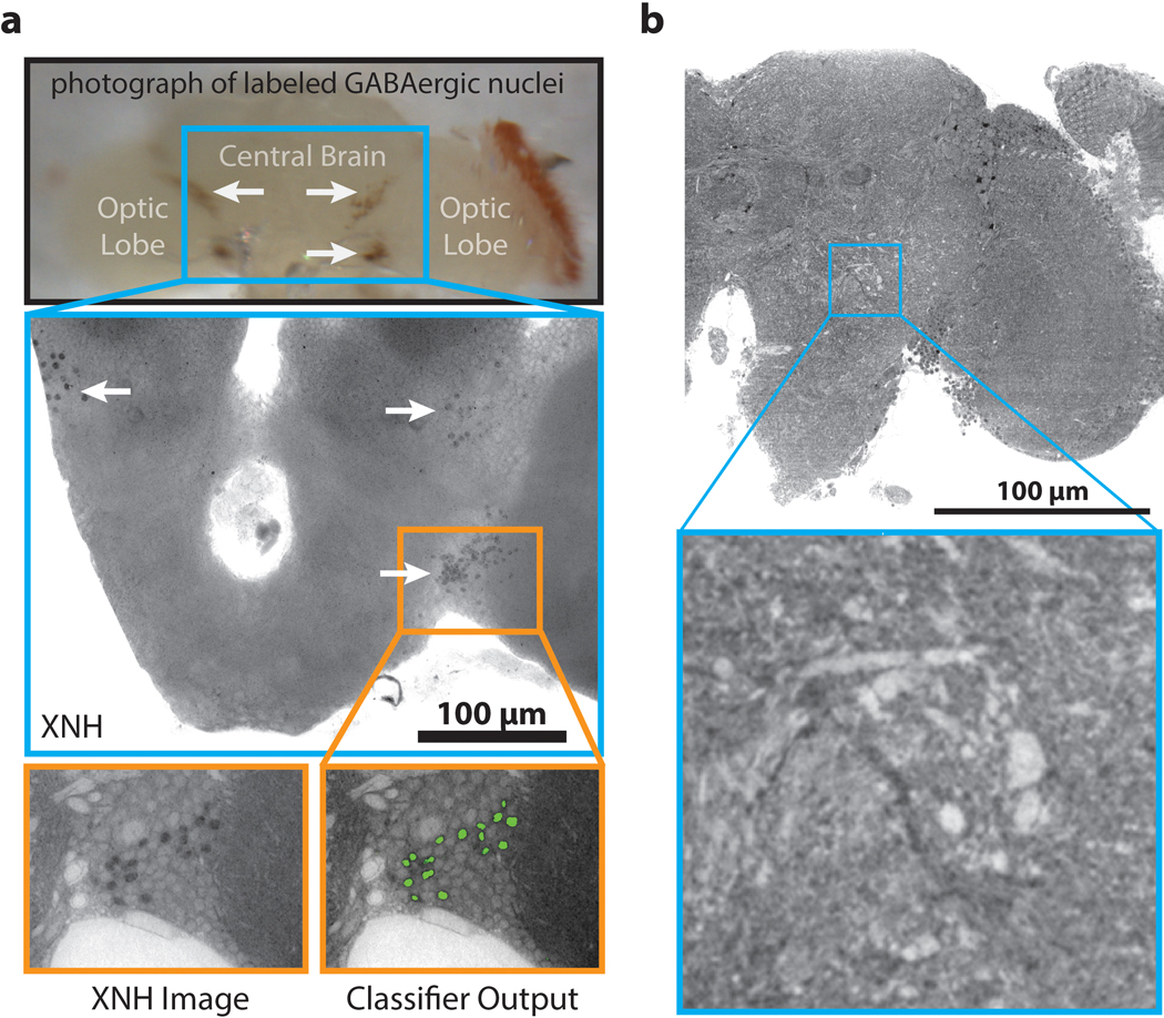
XNH and EM images, we reasoned that genetic labeling strategies previously developed for EM such as APEX2 52 , 54 could be adapted for XNH. We developed a fly reporter line that targets the peroxidase APEX2 54 to cell nuclei ( Methods ), and demonstrated that labeled neurons could be identified in XNH datasets (Extended Data Fig. 5a) . To target APEX2 to the nucleus, we fused a targeting sequence consisting of a methionine and 38 amino acids of the Stinger sequence (MSRHRRHRQRSRSRNRSRSRSSERKRRQRSRSRSSERRR) to APEX2. The targeting sequence was first cloned into the pENTR vector and subsequently cloned by recombination using the Gateway system into a destination vector (gift from Dr. Frederik Wirtz-Peitz) containing UAS-attR-sbAPEX2–3xMyc. The resulting UAS-NLS-APEX2-Myc construct was used to generate a transgenic line by direct injection using φC31 site-specific integration at the attP40 docking site on chromosome two. To test whether APEX2 labeled cells could be identified via XNH imaging, we labeled GABAergic nuclei with APEX2. Fly lines containing the transgenes Gad1-p65AD, UAS-CD8-GFP and elav-Gal4DBD, UAS-CD8-GFP (gifts from Dr. Haluk Lacin) were crossed with the nuclear-APEX2 fly described above to generate flies with genotype w; elav-Gal4DBD, UAS-CD8-GFP / UAS-NLS-APEX2-Myc; Gad1-p65AD, UAS-CD8-GFP / +. The nervous system from a 5–6 day old adult female fly was prepared for XNH imaging as described above. To automatically detect APEX2-labeled cell nuclei in XNH images, a 3D random forest pixel classifier was created, trained, and deployed using ilastik 55 . For training, a sparse set of pixel labels was interactively annotated for background pixels and labeled cell body pixels. See Life Sciences Reporting Summary for more details.
Experimental setup and data acquisition
XNH imaging was performed at beamline ID16A at the European Synchrotron in Grenoble, France. The end-station of the beamline is placed 185 m from the undulator source for improved coherence. The X-ray beam was focused using fixed curvature, multilayer coated Kirkpatrick-Baez mirrors into a spot measuring about 15 nm at X-ray energy of 33.6 keV 23 and 30 nm at 17 keV. The photon flux was on the order of 1–4 × 10 11 ph/s. The sample stage and X-ray focusing optics were placed in a vacuum chamber (pressure ~10 −8 mbar) and a liquid nitrogen based cryogenic system was integrated inside the stage, keeping the sample at 120 K during imaging. For cryogenic imaging, the samples were transferred into the vacuum chamber with a Leica cryo-shuttle. The samples were placed on a high-precision rotation stage 56 downstream of the beam focus, and intensity projections (i.e. holograms) were recorded using a FReLon 4096 × 4096 pixel CCD detector 57 with 2x binning, lens-coupled to a 23 μm thick GGG:Eu scintillator. After traversing the sample, the beam was allowed to propagate and generate self-interference patterns (i.e. holograms). The resulting intensity was recorded on the detector placed 1.2 m downstream of the sample. The divergent beam gives geometrical magnification M = (z 1 + z 2 )/z 1 with z 1 = focus-to-sample distance and z 2 = sample-to-detector distance. Therefore, the pixel size and the corresponding FOV are proportional to z 1 when the detector position is fixed ( Fig. 1b ). For each scan, four tomographic series of projections (rotations of the sample over 180º) were recorded at different focus-to-sample distances. To eliminate ring artifacts in tomographic reconstructions, the samples were laterally displaced at each rotation angle by a randomly-determined distance of up to 25 pixels using high-precision piezoelectric actuators 24 . For each tomographic scan of the mouse cortex, 1800 projections were recorded with exposure times of 0.1 s at X-ray energy 17 keV and 0.35 s at 33.6 keV. For the Drosophila scans at 17 keV, 2000 projections were collected with 0.2 s exposure times.
Image reconstruction
The recorded holograms were initially preprocessed to compensate for distortions and noise specific to the optics and detector, and normalized with the empty beam 24 . For each rotation angle, the four holograms corresponding to different propagation distances were aligned and brought to the same magnification. Normally, the holograms are cropped to the smallest FOV, corresponding to the targeted pixel size. In order to obtain an extended FOV, the information from the three larger FOVs at lower resolutions was integrated in the reconstruction as well. From these sets of aligned holograms, phase maps were obtained through an iterative algorithm 21 , 58 – 60 . The initial approximations of the amplitude and phase were obtained through a method based on 61 , adapted for multiple propagation distance holograms 59 . For regularization we used the ratio between the refractive index decrement δ and the absorption index β corresponding to Osmium (δ/β = 27 for X-ray energy 33.6 keV and δ/β = 9 for 17 keV). This regularization was used only to obtain the starting point of the iterative approach and only affects low spatial frequencies. At each iterative step, the amplitude term was kept constant and the phase term was updated. Typically, 10 iterations were sufficient for the phase term to converge. Computation time was approximately 15 minutes per phase map (single CPU node). Computation of the phase maps was done in parallel by treating the holograms for each rotation angle independently. Lastly, a 3D image volume of the tissue was generated by combining the phase maps from all angles into a tomographic reconstruction using filtered back-projection 62 . Iterative CT approaches and regularization were not used here. Since we acquire and combine four sets of angular projections at four different geometrical magnifications, we can use the lower resolution – larger FOV information to reconstruct extended FOV tomograms. In this case the reconstructed volume is larger than the detector size ( Supplementary Data Table 1 ), however, the image quality degrades gradually towards the edges of the extended field since less information is available (Extended Data Fig. 1d) .
Resolution Measurements
While the voxel size is directly determined by the sample positioning, the effective resolution depends on multiple factors, including the focal point size and the coherence properties of the X-ray beam, mechanical stability, detector characteristics, sample composition and image reconstruction approach. To measure the effective resolution, we used Fourier Shell Correlation and Edge-Fitting independently (see below), and found the results to be consistent.
Fourier Shell Correlation
To perform Fourier Shell Correlation (FSC) 25 , we split the data into two independently-acquired image volumes (see below) and measured the normalized cross-correlation coefficient between the two volumes over corresponding shells (size 6) in Fourier space. The intersection between the FSC line and the ½-bit threshold 63 was used to determine the resolution (Extended Data Fig. 1c) . The two image volumes were generated independently from half of the phase maps (even and odd phase projections were separated). FSC was applied by comparing chunks from the two image volumes at corresponding locations. The size of these chunks was varied to find a size at which the FSC metric was stable, which occurred at chunk sizes of ~200 3 voxels or larger. Measurements on larger chunks (up to 1000 3 voxels) remained stable, but took longer to compute. Computation was performed on evenly spaced chunks across the volume, excluding the regions containing only empty resin. Once the resolutions for all chunks were measured, the median and IQR were calculated ( Fig. 1h , Extended Data Fig. 1b ). For characterization of resolution within a single scan (Extended Data Fig. 1d) , FSC was performed on image cubes containing 100 3 voxels, and each cube was plotted separately. Edge-Fitting For measuring resolution by edge-fitting, line paths perpendicular to sharp edges in the image volumes were annotated manually using CATMAID ( Extended Data Fig. 1e , f , left) 45 , 64 . The image intensity along these line paths were then calculated using the pyMaid python API ( https://github.com/schlegelp/pyMaid ). The points along the line paths were fit to the sigmoid function: p 3 + p 0 2 ( 1 − t a n h ( x − p 1 p 2 ) ) Where x is the length along the line path and p 1 – 4 are free parameters determined by nonlinear regression. ( Extended Data Fig. 1e , f , middle). Given a fit to an edge, the measured resolution is given by: r e s = a s e c h ( 2 2 | p 2 | ) The fits to each line path were inspected and poor fits were refit with different initial parameters or removed. Edge-fitting was used in the 30 nm mouse cortex dataset ( Extended Data Fig. 1e ) and the 50 nm Drosophila VNC dataset ( Extended Data Fig. 1f ). For each dataset, 30 measurements were taken ( Extended Data Fig. 1e , f , right). For purposes of comparison, we also applied edge-fitting measurements to electron microscopy images of thin-sections of Drosophila VNC ( Extended Data Fig. 1g , 4 nm pixels, 45 nm thick section). Variability in Measured Resolution In XNH data, resolution is generally better for scans with smaller voxel size ( Fig. 1h ). However, measured resolution was significantly larger than the voxel size, between 1.5 to 3.5 times the voxel size. In EM images of nervous tissue, the ratio of measured resolution to pixel size is similar ( Extended Data Fig. 1g ). As the voxel size is reduced, the resolution per voxel deteriorates ( Extended Data Fig. 1b ). This is due to a combination of factors, such as more challenging conditions for phase retrieval and tomographic reconstruction and higher risk of sample warping during the scan. The photon flux density increases with smaller voxel sizes, so limiting the radiation dose and imaging at cryogenic temperatures are more critical. Sample to sample differences also affect the resolution. Sample density can affect beam absorption and heating, and the location of the field of view relative to the mounting pin can affect heat dissipation. For one sample (fly leg), we imaged the same field of view with different voxel sizes, and found that the measured resolution improved monotonically with smaller voxel size (Extended Data Fig. 1h) . We found that the measured resolution is approximately uniform across the scan volumes (i.e. the tomographic reconstruction does not introduce major anisotropy in the image quality) ( Extended Data Fig. 1d ). However, the resolution near the axis of rotation (the center of the cylinder) appears slightly better. Also, areas in extended field of view (areas outside the detector size, beyond red line in Extended Data Fig. 1d ) exhibit slightly degraded resolution. There may also be variation in measured resolution intrinsic to the evaluation method. For example, regions of empty resin (devoid of structure) within a sample exhibit poor resolution when measured by FSC. These regions were excluded from FSC calculations ( Fig. 1h , Extended Data Fig. 1b , Supplementary Data Table 1 ).
Post-Hoc EM imaging
After completing XNH imaging, samples were re-embedded in a block of resin and trimmed for thin-sectioning. Serial thin sections (45–100 nm) were cut using a 35 degree diamond knife (Diatome) and collected onto LUXFilm-coated copper grids (Luxel Corp.). Sections were imaged on a JEOL 1200EX transmission electron microscope (80 kV accelerating potential, 1500x mag), and images were acquired with a 20 MPix camera system (AMT Corp.) at 4–12 nm pixels. For the fly VNC sample, several thin sections including the main leg nerve were collected and imaged with TEM ( Fig. 1i ). The XNH image volume was rotated to match the orientation of the transmission EM (TEM) sections using Neuroglancer ( https://github.com/google/neuroglancer ). The TEM image of the leg nerve was elastically aligned to a single matching image taken from the XNH dataset using AlignTK ( https://mmbios.pitt.edu/aligntk-home ). Neurons in corresponding images from XNH and EM were independently segmented using the manual annotation software ITK-snap 65 ( www.itksnap.org ) ( Fig. 1i , Extended Data Fig. 1i ). The segmentation generated from the EM image was taken as ground truth, and the accuracy of the XNH segmentation was calculated by comparing it to the EM segmentation. For each neuron, segmentation was considered correct if the number of overlapping pixels shared between the EM and XNH segmentation was greater than half of the number of pixels for the neuron in both XNH and EM segmentations ( Extended Data Fig. 1i , right). The size of each neuron was approximated as the diameter of the largest circle centered at the neuron’s center of mass that could fit entirely within the neuron ( Extended Data Fig. 1j ). Note that this analysis used only 2D image data – additional 3D information would likely improve performance. For the posterior parietal cortex sample, a 3D EM dataset in posterior parietal cortex ( Fig. 2 ) was collected and imaged using the GridTape pipeline for automated serial section transmission EM 66 . To find the region of tissue imaged with XNH, 1 μm thick histological sections were collected and compared with XNH virtual slices. 250 thin sections (~45 nm thick) were collected onto GridTape for a total of 11 μm total thickness. For each section, an ROI overlapping with the XNH imaged region was imaged using a customized JEOL 1200EX TEM outfitted with a reel-to-reel GridTape stage. Total EM imaging time was approximately 150 hours. In the EM images, the tissue ultrastructure, including chemical synapses, remained well-preserved after XNH imaging ( Extended Data Fig. 2b , inset, arrows). The EM images also contained small cracks (orange arrows) and bubbles (inset, pink arrows), which may have resulted from XNH imaging. These minor artifacts did not affect our ability to analyze the data, but it is possible that they can be reduced or eliminated by modifying XNH imaging protocols. However, more correlative XNH-EM data is needed to understand the origin of microcracks and nanobubbles. The EM images were stitched together and aligned into a continuous volume using the software AlignTK ( https://mmbios.pitt.edu/software#aligntk ). The XNH datasets were aligned to the EM volume via an affine transformation based on manually annotated correspondence points (annotated using BigWarp https://imagej.net/BigWarp ). Data annotation (tracing of apical dendrite morphologies and annotation of synapses) was done with CATMAID 45 , 64 .
Image Volume Stitching
For each pair of XNH scan volumes with overlapping FOVs, correspondence points identifying the same feature in each scan were annotated manually using the ImageJ plugin BigWarp 67 ( https://imagej.net/BigWarp ). Translation-rotation-scaling matrices were calculated based on least-squares fitting of these correspondence points (~10–20 pairs per image volume) using custom MATLAB code, then applied to each image volume using the ImageJ plugin BigStitcher 68 . To avoid blurring from misalignments in regions where two scans overlap, image volumes were combined without blending in overlapping regions (custom Python code).
Data analysis – Posterior Parietal Cortex
Manual tracing of neurons was performed by a team of 2 annotators using CATMAID 45 , 64 . All cell somata within the XNH volume were identified manually and classified as non-neuronal, pyramidal neuron, or inhibitory neuron ( Fig. 2e , Extended Data Fig. 2c ) 30 , 69 , 70 . For a subset of pyramidal neurons distributed across layers II, III, and V, the apical dendrites were traced in the XNH volume up towards the superficial layers until they intersected the EM volume ( Fig. 2b , Fig. S2e ). The same apical dendrites were then identified in the EM volume based on their location and shape ( Fig. S2b ). Within the EM volume, all incoming synapses to the apical dendrite were annotated as excitatory (targeting dendritic spines) or inhibitory (targeting dendritic shafts or spine necks) ( Fig. 2d ). Presynaptic axons, which were resolvable in the EM data but not the XNH data, were not traced. Pyramidal cells were classified as layer II, III, or V based on the distance of their cell body from the layer I/II boundary, which was estimated as a plane above which the density of cell somata drops dramatically ( Fig. 2b , Extended Data Fig. 2a ). All tracing was reviewed independently by a second annotator to ensure accuracy. To calculate synapse densities, we wrote custom python code utilizing the pyMaid python API ( https://github.com/schlegelp/pyMaid ) to access the CATMAID database. The calculate synapse densities for a given AD ( Fig. 2f ), the total number of inhibitory or excitatory synapses found in the EM volume was divided by the total pathlength of the AD within the EM volume. For these analyses the location of the excitatory synapses was defined as the location of the base of the spine neck, and only the dendrite trunk (excluding the spines) was used for calculating the dendrite pathlength. The inhibitory synapse fraction was defined as (# inhibitory synapses / total # of synapses). To calculate synapse densities as a function of AD pathlength ( Fig. 2h – i , Extended Data Fig. 2g – h ), each AD was split into fragments 10 μm in length, and the synapse densities were calculated for each fragment individually. The AD pathlength was defined as the along-the-arbor distance from the center of the dendrite fragment to the soma ( Fig. 2h – i ) or initial bifurcation ( Extended Data Fig. 2g – h ).
Data analysis – Drosophila leg and VNC
Sensory receptors, muscle fibers, and neurons were annotated manually using CATMAID 45 , 64 . Sensory receptors and muscle fibers were large enough to be clearly resolved in the XNH volume (50–75 nm voxels). Larger axons were also clearly resolved throughout the leg and VNC (motor neurons, coxal hair plate neurons, trochanteral campaniform sensilla neurons), but other smaller axons (bristle neurons in particular) were too small to be accurately traced. 3D visualizations were produced using ITK-SNAP ( Fig. 2c ), the 3D viewer widget in CATMAID ( Fig. 3 , Extended Data Fig. 2e , Extended Data Fig. 3e , f , g , m , n , Extended Data Fig. 4d , ), Neuroglancer ( Fig. 4 , Extended Data Fig. 4j , k ), Paraview ( Fig. 1e , Extended Data Fig. 3a ) or Fiji ( Fig. 1f , Extended Data Fig. 3c ).
Automated Segmentation
We used an automated segmentation workflow based on a segmentation pipeline for TEM data 41 . The pipeline consists of two major steps: affinity prediction and agglomeration. In the affinity prediction step, a 3D U-Net convolutional neural network (CNN) was used to predict an affinity graph from the image data. The value of the affinity graph at any given voxel represents a pseudo-probability that adjacent voxels (in the x, y, and z axes) are part of the same object. Adjacent voxels crossing object boundaries should have low affinity values, whereas voxels within neurons should have high affinity to the voxels surrounding them (including voxels contained in organelles or other subcellular structures).
Network Training
To expedite training a CNN on XNH data, we leveraged a CNN first trained on ground truth EM volumes from the CREMI challenge ( https://cremi.org/ ), followed by training augmentation with corrected segmentation predicted on XNH data. We began by training an initial network on the CREMI ground truth data (4 nm x 4 nm x 40 nm) downsampled to match the voxel size of the XNH data (50 nm x 50 nm x 50 nm). We deployed this CREMI-trained network on a training volume of XNH data (320 × 320 × 300 voxels) and used Armitage/BrainMaps (Google) to correct the voxelwise segmentation for a sparse set of neurons. The network was then deployed on two more training volumes (200 × 200 × 200 voxels, one in the main leg nerve, one in the T1 neuropil) which were densely traced (via skeletonization, not voxel-wise) by human annotators (using CATMAID). Skeleton tracing was used in lieu of voxel-wise error-correction because it can be completed in much less time and is less likely to introduce human errors in the training volumes. The tracing in these training volumes was used to correct errors in the candidate segmentation, and the corrected training volumes were then used to train the network further, resulting in the final network. The final network was then deployed on the entire dataset. Deploying the network on a server that has 40 CPU cores and ten NVIDIA GTX 2080 Ti’s across the full dataset (1792 × 3584 × 3200 voxels) took less than 10 minutes. Neuron reconstruction and proofreading We developed a proofreading workflow based on Neuroglancer ( https://github.com/google/neuroglancer ) to rapidly reconstruct and error correct neurons from automated segmentation. Although split and merge errors exist in the automated segmentation, such errors are usually easy for humans to recognize in 3D visualizations of reconstructed neurons. Thus, proofreading automated segmentation results is much faster than manual tracing. For reconstruction/proofreading, a blocked segmentation methodology (in which the volume was divided into independent blocks of 256 3 voxels) was used. Neurons were seeded by selecting a neuron fragment (contained within a single block) in the main leg nerve, and sequentially grown by adding neuron fragments in adjacent blocks. During each growth step, the 3D morphology of the neuron was visualized and checked for errors. When merge errors occur, the blocks containing the merge are “frozen” to prevent growth from the merged segment. When a neuron branch stops growing (has no continuations), the proofreader inspects the end of the branch to check from missed continuations (split errors). In this way, both split and merge errors can be corrected. In the fly VNC XNH dataset, neurons took about 10–30 min each to reconstruction/proofread.
Neuron classification
Neurons were classified as motor neurons or sensory neuron subtypes by based on their location in the nerve and 3D morphology 40 , 42 , 43 , 71 . The reconstructed neurons are likely missing branches or continuations where they become too small to be resolved XNH. However, in most cases, the large-scale branching patterns were sufficient to classify the neurons. 166 neurons were reconstructed from seeds within the main leg nerve, out of which 66 were not clearly classified into a subtype and were excluded from Fig. 4f and Extended Data Fig. 4c . These unclassified neurons tended to be small fragments that do not extend significantly into the VNC, typically because they became too small to be reliably segmented (see also Extended Data Fig. 1i – j ).
Segmentation error quantification
To access the accuracy of automated segmentation, we manually traced 90 neurons from the XNH data (CATMAID) and compared them to the automated segmentation results. For each neuron, a list of all skeleton node (manually placed) – segmentation fragment ID (automatically generated) pairs was generated. In a perfect segmentation, all skeleton nodes for a given skeleton would correspond to the same segmentation ID. For each manually-generated skeleton (neuron), a split error was counted for each extra segmentation ID associated with nodes in that skeleton. Split errors that did not change the topology of the neuron were not counted. For each segmentation ID, a merge error was counted for each segmentation fragment that was paired with skeleton nodes from multiple different neurons. To accuracy the count the number of such merge errors, the blocked segmentation was used (see Neuron Reconstruction and Proofreading above). This way, if two neurons are merged in two different places, it will count as two merge errors. It is worth noting that in this calculation, merge errors are only counted between the subset of neurons for which we performed manual skeletonization. Therefore, if portions of nearby un-skeletonized neurons were merged into the segmentation of a skeletonized neuron, that error would not be detected here. Visual inspection of the segmentation results suggest that this type of error is not overly common, but nevertheless the counts of merge errors reported here are likely an underestimate of the true rate of merge errors. It is important to note that in the neurons shown in Fig. 4f and Extended Data Fig. 4c , most split and merge errors were corrected via reconstruction/proofreading.
Statistics and Reproducibility
The quality of XNH reconstructions depended on imaging settings and sample characteristics, and was generally reproducible for a given set of parameters. For example, 8 XNH scans of the same fly leg sample were recorded with the same imaging parameters with similar results ( Supplementary Data Table 2 ). The 11 datasets reported in Fig. 1h , Supplementary Data Table 1 , and Supplementary Videos are a representative sample of XNH reconstruction quality over a range of imaging and sample parameters. Scans acquired during exploratory experiments which yielded poor quality data were not included for data analysis. For statistical analysis in Fig. 2 , the number of annotated neurons (n = 261) was calculated to ensure that a large number of sample points (> 30) exist in each of the 4 sublayers (IIa, IIb, III, V). No a priori statistical power calculations were performed to determine sample size but our sample sizes are larger than those reported in previous publications (ref. 27). For bootstrap analysis of variance ( Fig. 2f ), 1000 synthetic samples were generated from each layer (layer IIa, layer IIb, layer III, and layer V) by randomly selecting datapoints with replacement until the number matched the original dataset size. Then the mean synapse density or inhibitory synapse fraction was calculated for all 1000 synthetic samples. The plotted 95% confidence intervals plotted in Fig. 2f are the 2.5 th and 97.5 th percentile values from this distribution of synthetic sample means. This bootstrap analysis is a non-parametric test and does not assume normality or equal variances. EM micrographs shown in Fig. 1i and Extended Data Fig. 1i are representative images. 10 similar thin-sections were prepared and imaged with similar quality, although some sections showed physical damage sustained during the sectioning process. EM micrographs shown in Fig. 2d and Extended Data Fig. 2b are representative images. More than 2 million images with similar quality were recorded from this sample using automated EM, although some regions exhibited small cracks and bubbles, which may have been caused by prior XNH imaging. This study involved detailed anatomical analysis of nervous tissue samples. In most analyses, were examined fundamental organizational principles of neuronal morphology and connectivity, rather than comparing experimental and control samples. Therefore, randomization was not necessary. Our data was not allocated into groups, thus blinding was not applicable; Data collection and analysis were not performed blind to the conditions of the experiments. See Life Sciences Reporting Summary for more details.
Experimental Animals
Experimental procedures were approved by the Harvard Medical School Institutional Animal Care and Use Committee and performed in accordance with the Guide for Animal Care and Use of Laboratory Animals and the animal welfare guidelines of the National Institutes of Health.
Mice
(Mus musculus) used in this study were C57BL/6J-Tg(Thy1-GCaMP6s)GP4.3Dkim/J, male, 32 weeks and C57BL/6, male, 28 weeks, ordered through Jackson Laboratory (The Jackson Laboratory, Bar Harbor, ME). Mice were housed up to 4 per home cage at normal temperature and humidity on reverse light cycle, and relocated to clean cages every two weeks. Flies ( Drosophila melanogaster ) used in this study were 1–7 day old female adults with the w1118 genetic background. The transgenic approach for labeling GABAergic nuclei (used in Fig. 3 and Extended Data Fig. 5 ) is described below. See Life Sciences Reporting Summary for more details.
Experimental setup and data acquisition
XNH imaging was performed at beamline ID16A at the European Synchrotron in Grenoble, France. The end-station of the beamline is placed 185 m from the undulator source for improved coherence. The X-ray beam was focused using fixed curvature, multilayer coated Kirkpatrick-Baez mirrors into a spot measuring about 15 nm at X-ray energy of 33.6 keV 23 and 30 nm at 17 keV. The photon flux was on the order of 1–4 × 10 11 ph/s. The sample stage and X-ray focusing optics were placed in a vacuum chamber (pressure ~10 −8 mbar) and a liquid nitrogen based cryogenic system was integrated inside the stage, keeping the sample at 120 K during imaging. For cryogenic imaging, the samples were transferred into the vacuum chamber with a Leica cryo-shuttle. The samples were placed on a high-precision rotation stage 56 downstream of the beam focus, and intensity projections (i.e. holograms) were recorded using a FReLon 4096 × 4096 pixel CCD detector 57 with 2x binning, lens-coupled to a 23 μm thick GGG:Eu scintillator. After traversing the sample, the beam was allowed to propagate and generate self-interference patterns (i.e. holograms). The resulting intensity was recorded on the detector placed 1.2 m downstream of the sample. The divergent beam gives geometrical magnification M = (z 1 + z 2 )/z 1 with z 1 = focus-to-sample distance and z 2 = sample-to-detector distance. Therefore, the pixel size and the corresponding FOV are proportional to z 1 when the detector position is fixed ( Fig. 1b ). For each scan, four tomographic series of projections (rotations of the sample over 180º) were recorded at different focus-to-sample distances. To eliminate ring artifacts in tomographic reconstructions, the samples were laterally displaced at each rotation angle by a randomly-determined distance of up to 25 pixels using high-precision piezoelectric actuators 24 . For each tomographic scan of the mouse cortex, 1800 projections were recorded with exposure times of 0.1 s at X-ray energy 17 keV and 0.35 s at 33.6 keV. For the Drosophila scans at 17 keV, 2000 projections were collected with 0.2 s exposure times.
Supplementary Material Supplemental Material 1618914_Reporting summary 1618914_Supp_vdo1 1618914_Supp_vdo2 1618914_Supp_vdo3 1618914_Supp_vdo4 1618914_Supp_vdo5 1618914_Supp_vdo6 1618914_SD_fig
📊 Figures
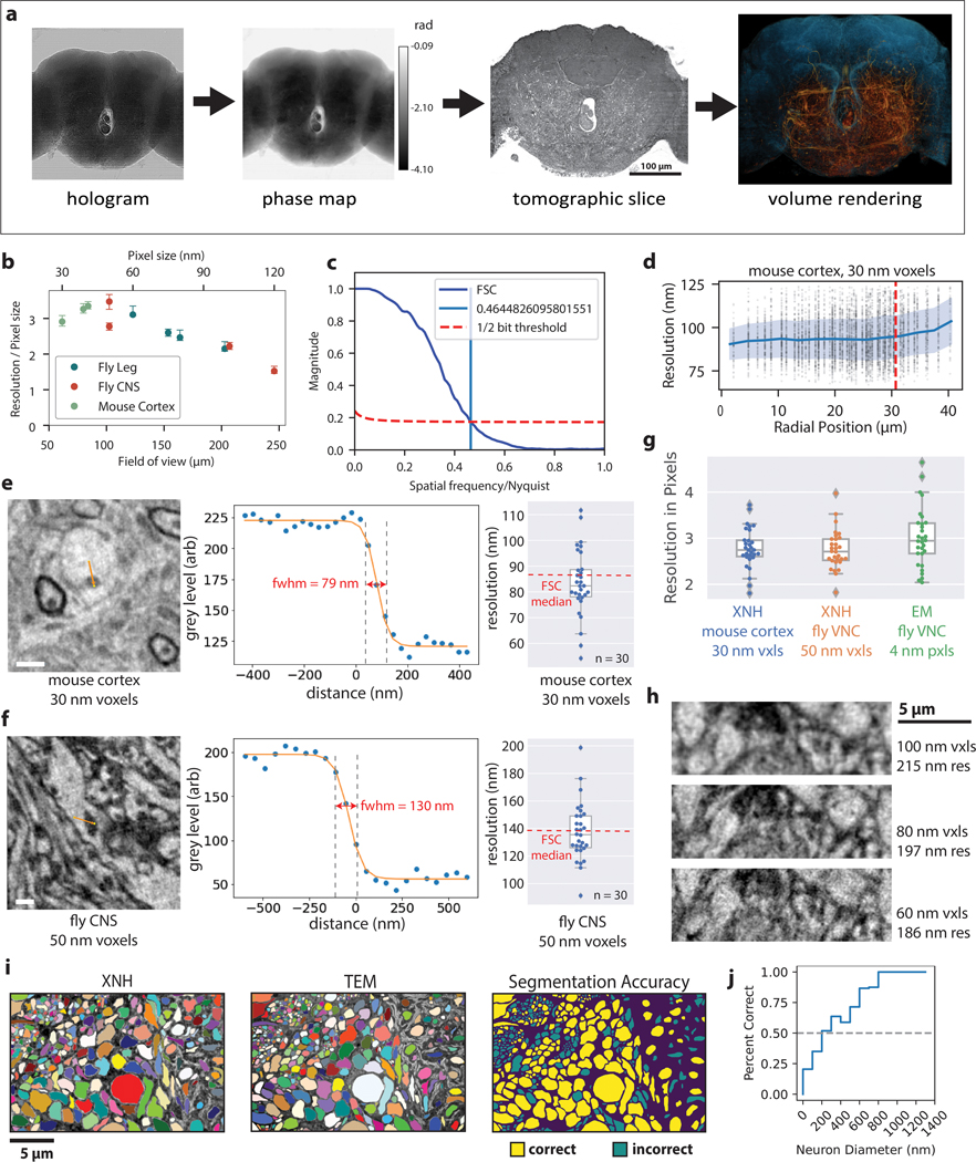
Extended Data Figure 1:
X-ray Holographic Nano-Tomography (XNH) Technique and Characterization.
(a) Overview of XNH imaging and preprocessing. Left: Holographic projections of the sample (a result of free-space propagation of the coherent X-ray beam) are recorded for each angle as the sample is ...
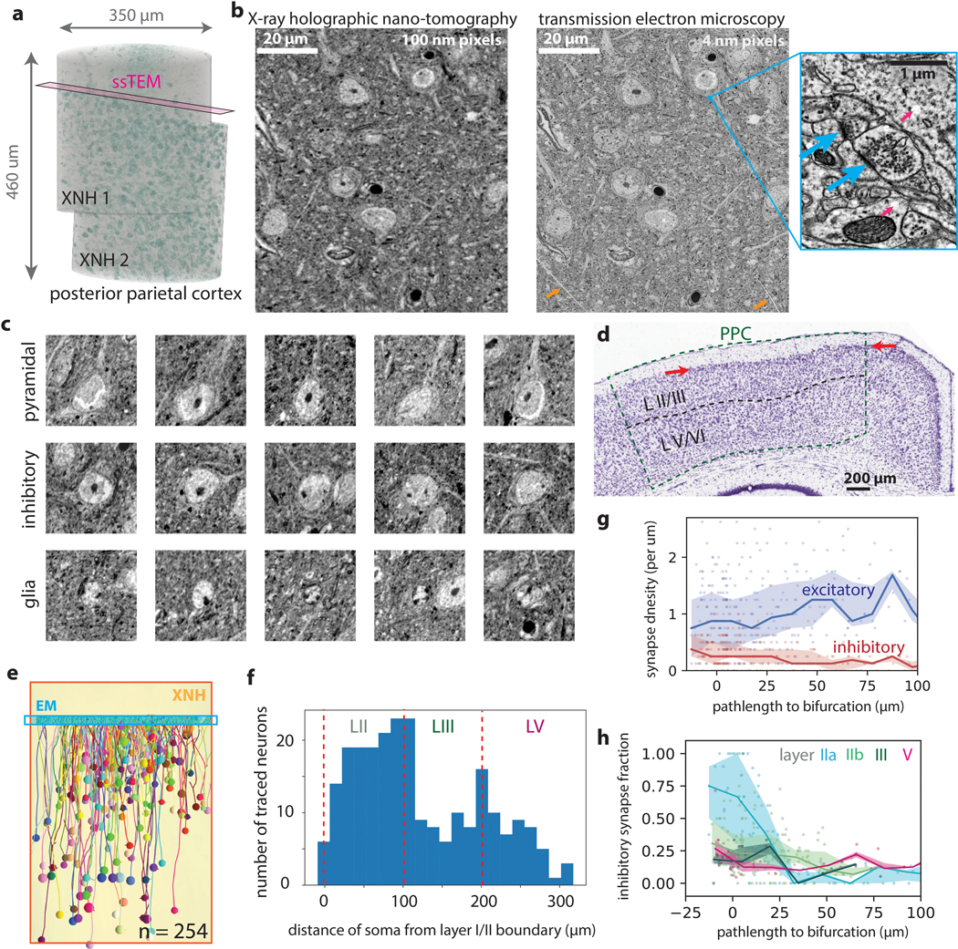
Extended Data Figure 2:
Correlative XNH - EM analysis of the connectivity statistics of pyramidal apical dendrites in posterior parietal cortex (PPC).
(a) 3D rendering of two aligned and stitched XNH datasets in mouse posterior parietal cortex. Cell somata are colored in green (based on voxel brightness). Magenta plane indicates location of serial E...
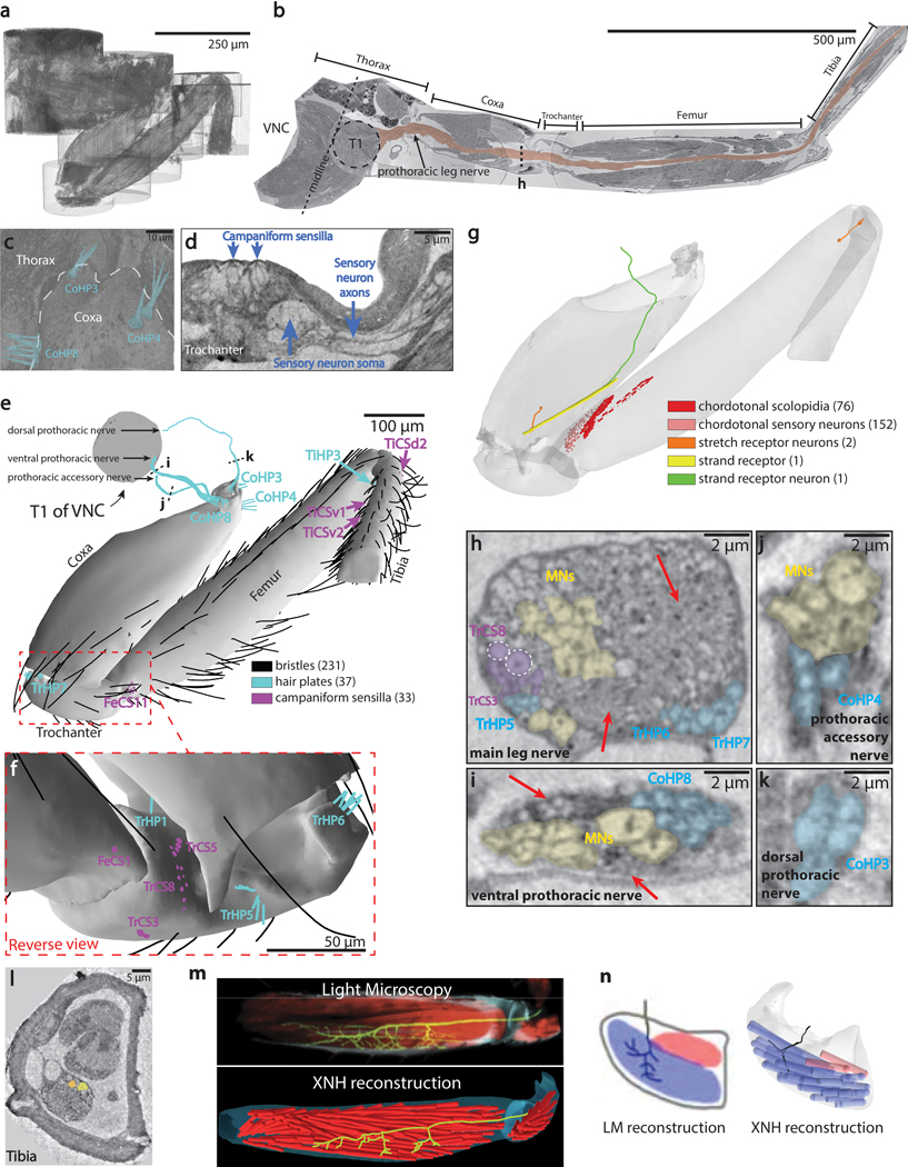
Extended Data Fig. 3:
Millimeter-scale imaging of a Drosophila leg at single-neuron resolution.
(a) 3D rendering of the dataset after individual scans were stitched together to form a continuous volume. ( b ) The image volume was computationally unfolded (ImageJ) to reveal the entire 1.4mm lengt...
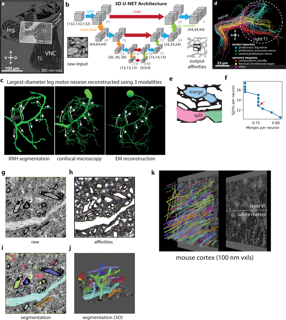
Extended Data Figure 4:
Automated Segmentation of Neuronal Morphologies using Convolutional Neural Networks (CNNs).
(a) Overview of XNH image volume encompassing the anterior half of the VNC and the first segment of a front leg of an adult Drosophila (200 nm voxels). A smaller, higher resolution (50 nm voxels) volu...
Extended Data Figure 5:
Additional staining approaches for XNH imaging.
(a) Top: Photograph of fly brain with GABAergic nuclei labeled with APEX2 (arrows). Middle: XNH images (120 nm pixels, 15 u03bcm thick minimum intensity projection) of the same fly brain after heavy m...
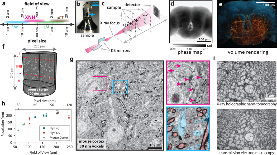
Figure 1:
X-ray Holographic Nano-Tomography (XNH) Technique and Characterization.
(a) Schematic depicting pixel and FOV sizes for XNH imaging, along with comparisons to other modalities (assumes a 4 Mpixel detector). Note that EM imaging is generally performed on thin sections or s...
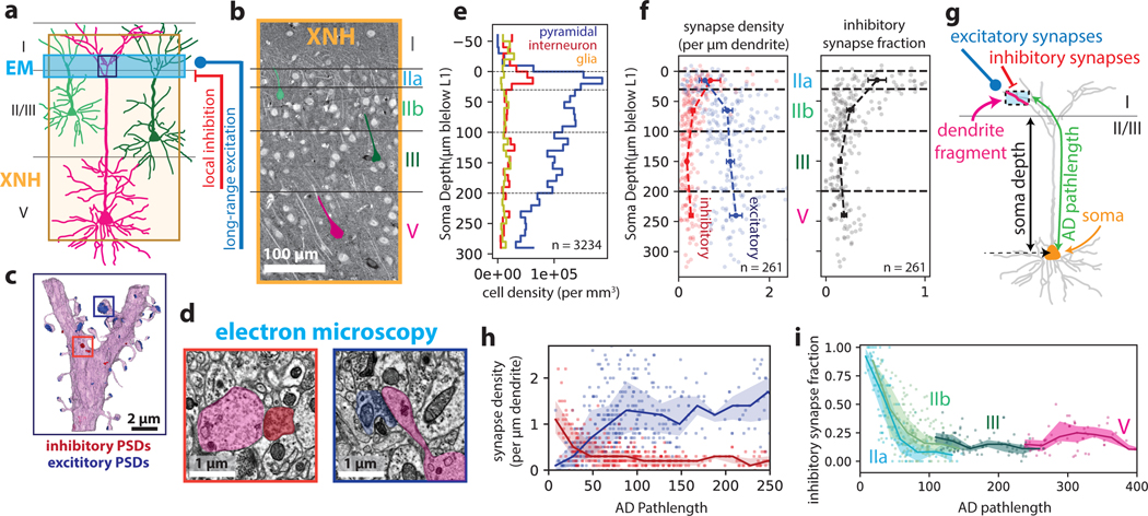
Figure 2:
Correlative XNH - EM analysis of the connectivity statistics of pyramidal apical dendrites in posterior parietal cortex (PPC).
(a) Experimental approach: XNH imaging covers superficial and deep layers of PPC with sufficient resolution to resolve cell bodies and apical dendrites (ADs). Targeted 3D EM volume captures the layer ...
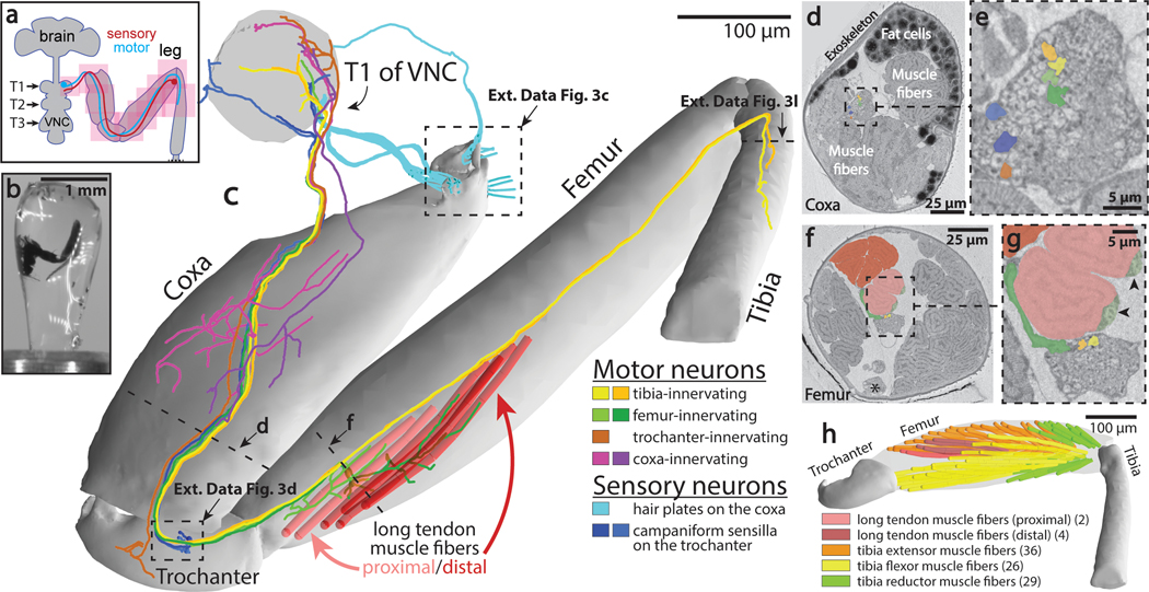
Figure 3:
Millimeter-scale imaging of a Drosophila leg at single-neuron resolution.
(a) Schematic of XNH imaging strategy. Ten partially-overlapping XNH scans ( Supplementary Data Table 2 ) were used to capture a front legu2019s coxa, trochanter, femur, and half of the tibia, plus th...
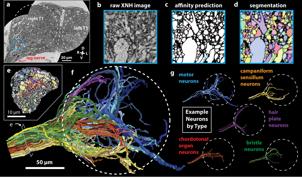
Figure 4:
Automated Segmentation of Neuronal Morphologies using Convolutional Neural Networks (CNNs).
(a-b) Raw XNH image data, recorded from the T1 neuromeres of an adult Drosophila VNC. V, ventral; D, dorsal; R, right; L, left. (c) Predicted affinities output by a 3D U-NET ( Extended Data Figure 4b ...
Figure images are served from the NIH/NLM PubMed Central Open Access Subset or Europe PMC; copyright remains with the publishers and authors.
💬 Discussion
0 commentsNo comments yet. Be the first to start a discussion!
Leave a Comment