Abstract
Deciding between stimuli requires combining their learned value with one's sensory confidence. We trained mice in a visual task that probes this combination. Mouse choices reflected not only present confidence and past rewards but also past confidence. Their behavior conformed to a model that combines signal detection with reinforcement learning. In the model, the predicted value of the chosen option is the product of sensory confidence and learned value. We found precise correlates of this variable in the pre-outcome activity of midbrain dopamine neurons and of medial prefrontal cortical neurons. However, only the latter played a causal role: inactivating medial prefrontal cortex before outcome strengthened learning from the outcome. Dopamine neurons played a causal role only after outcome, when they encoded reward prediction errors graded by confidence, influencing subsequent choices. These results reveal neural signals that combine reward value with sensory confidence and guide subsequent learning.
🔬 Techniques
🔭 Microscopes
💻 Software
✨ Fluorophores
🧪 Sample Preparation
🏭 Microscope Brands
🧪 Reagent Suppliers
📷 Detectors
💻 Software Details
💻 Code & Software
💾 Data Repositories
🏷️ Research Resource Identifiers (RRIDs)
Verified research resources used in this paper:
🏛️ Research Organizations (ROR)
Affiliated research institutions:
📋 Methods
Key Resources Table
REAGENT or RESOURCE SOURCE IDENTIFIER Antibodies Primary Anti-TH Newmarket Scientific 22941 Secondary Alexa Goat anti-mouse conjugate (Alexa Fluor 594) Life-Tech A-11032 Anti-GFP antibody Abcam ab6556 Alexa Goat Anti RABBIT (Alexa Fluor 488) Life-Tech A-11034 Alexa Goat anti-mouse conjugate (Alexa Fluor 594) Life-Tech A-11032 Virus Strains AAV1.Syn.Flex.GCaMP6m.WPRE.SV40 Penn Vector Core N/A AAV5.EF1a.DIO.hChr2(H134R)-eYFP.WPRE Gift from Karl Deisseroth (Addgene viral prep # 20298_AAV5); http://addgene.org/20298 ; RRID:Addgene_20298) 20298_AAV5 rAAV5/EF1a-DIO-eArch3.0-eYFP University of North Carolina Vector Core N/A Mice C57/BL6J N/A N/A B6.SJLSlc6a3tm1.1(cre)Bkmn/J Jax 6660 B6.129P2-Pvalb tm1(cre)Arbr /J Jax 8069 Software and Algorithms MATLAB Mathworks 2016 ImageJ NIH https://imagej.nih.gov/ij Signals https://github.com/dendritic/signals N/A Lead Contact and Materials Availability Further information and requests should be directed to and will be fulfilled by the Lead Contact, Armin Lak ( armin.lak@dpag.ox.ac.uk ). This study did not generate new unique reagents.
Experimental Model and Subject Details
The data presented here was collected from 33 mice (19 male) aged between 10-24 weeks. Wild-type C57/BL6J mice, DAT-Cre mice backcrossed with C57/BL6J mice (B6.SJLSlc6a3tm1.1(cre)Bkmn/J) and Pvalb-Cre mice backcrossed with C57/BL6J (B6.129P2-Pvalb tm1(cre)Arbr /J) were used. All experiments were conducted according to the UK Animals Scientific Procedures Act (1986) under appropriate project and personal licenses.
Method Details Surgeries
All mice were first implanted with a custom metal head plate. To do so, the animals were anesthetized with isoflurane, and were kept on a feedback-controlled heating pad (ATC2000, World Precision Instruments, Inc.). Hair overlying the skull was shaved and the skin and the muscles over the central part of the skull were removed. The skull was thoroughly washed with saline, followed by cleaning with sterile cortex buffer. The head plate was attached to the bone posterior to bregma using dental cement (Super-Bond C&B; Sun Medical). For electrophysiological experiments, we covered the exposed bone with Kwik-Cast (World Precision Instruments, Inc.), trained the animals in the behavioral task in the following weeks, and subsequently performed a craniotomy over the frontal cortex for lowering the silicon probes. For fiber photometry and optogenetic experiments, after the head plate fixation, we made a craniotomy over the target area (mPFC or VTA) and injected viral constructs followed by implantation of the optical fiber, which was secured to the head plate and skull using dental cement. Post-operative pain was prevented with Rimadyl on the three following days. Behavioral tasks Behavioral training started at least 7 days after the head plate implantation surgery. For mice which received viral injection, training started 2 weeks after the surgery. Animals were handled and acclimatized to head fixation for 3 days, and were then trained in a 2-alternative forced choice visual detection task ( Burgess et al., 2017 ). After the mouse kept the wheel still for at least 0.5 s, a sinusoidal grating stimulus of varying contrast appeared on either the left or right monitor, together with a brief tone (0.1 s, 12 kHz) indicating that the trial had started. The mouse could immediately report its decision by turning the wheel located underneath its forepaws. Wheel movements drove the stimulus on the monitor, and a reward was delivered if the stimulus reached the center of the middle monitor (a correct trial), but a 2 s white noise was played if the stimulus reached the center of the either left or right monitors (an error trial). The inter trial interval was set to 3 s. As previously reported, well-trained mice often reported their decisions using fast stereotypical wheel movements ( Burgess et al., 2017 ). In the initial days of the training (first 4 to 7 days), stimuli had contrast = 1. Lower-contrast stimuli were introduced when the animal reached the performance of ∼70%. After 2-3 weeks of training, the task typically included 7 levels of contrast (3 on the left, 3 on the right and zero contrast) which were presented in a random order across trials with equal probability. We finally introduced unequal water rewards for correct decisions: in consecutive blocks of 50-350 trials (drawn from a uniform distribution), correct decisions to one side (left or right) were rewarded with larger reward (2.4 μL versus 1.2 μL of water) ( Figure 1 ). Experiments involving optogenetic manipulation of mPFC neurons or VTA dopamine neurons had the same timeline as described above ( Figures 4 and 5 ). In experiments involving fiber photometry, the task timeline slightly differed from above, allowing longer temporal separation of stimulus, action and outcome ( Figure 3 ). In these experiments, wheel movements immediately after the visual stimulus did not move the stimulus on the monitor and did not result in a decision (open-loop condition). Instead, an auditory go cue (0.1 s) which was played 0.6-1.8 s after the stimulus onset started the closed-loop during which animals could report the decision. Wheel movements prior to go cue did not terminate the trial and we did not exclude these trials from our analysis (excluding these trials did not affect our results). In these experiments, we defined the action time as the onset of first wheel movement after the stimulus onset. In all experiments, reaction times were measured from the onset of visual stimulus till the onset of the first wheel movement. The behavioral experiments were controlled by custom-made software written in MATLAB (Mathworks) which is freely available ( Bhagat et al., 2019 ). Instructions for hardware assembly are also freely available ( https://www.ucl.ac.uk/cortexlab/tools/wheel ). Electrophysiological experiments We recorded neuronal activity in prelimbic region of mPFC using multi-shank silicon probes in wild-type C57/BL6J mice. We implanted the animals after they fully learned to perform the task, performing the final stage of the behavioral task (including block switches) with performance above 70% for at least three sessions. A 32-channel, 2 shank silicon probe (Cambridge NeuroTech) was mounted on a moveable miniature Microdrive (Cambridge NeuroTech) and implanted it into mPFC (n = 6 mice). On the implantation day, we removed the Kwik-Cast cover from the skull and drilled a small incision in the cranium over the frontal cortex, ML = 0.3 mm, AP = 1.8 mm (burr #19007–07, Fine Science Tools). The brain was protected with Ringer solution. We lowered the probe through the intact dura using a manipulator (PatchStar, Scientifica) to 1.4 mm from the dura surface. The final approach toward the target depth (the last 100–200 μm) was performed at a low speed (2–4 μm/sec), to minimize potential damage to brain tissue. Once the probe was in its required position, we waited 10 minutes to let the brain recover from the insertion and fixed the Microdrive on the head plate using dental cement. For reference signal we used a skull screw implanted on the skull ∼3-4 mm posterior to the recording site. At the end of each recording day we lowered the Microdrive 100 μm. Recordings were performed using OpenEphys system. Broadband activity was sampled at 30 kHz (band pass filtered between 1 Hz and 7.5 kHz by the amplifier) and stored for offline analysis. Recorded spikes were sorted with KlustaSuite ( Rossant et al., 2016 ). Manual spike sorting was performed oblivious to task-related responses of the units. Fiber photometry experiments To measure the activity of dopamine neurons, we employed fiber photometry ( Gunaydin et al., 2014 , Lerner et al., 2015 ). We injected 0.5 μL of diluted viral construct (AAV1.Syn.Flex.GCaMP6m.WPRE.SV40) into the VTA:SNc (ML:0.5 mm from midline, AP: −3 mm from bregma and DV:-4.4 mm from the dura) of DAT-Cre mice backcrossed with C57/BL6J mice (B6.SJLSlc6a3tm1.1(cre)Bkmn/J). We implanted an optical fiber (400 μm, Doric Lenses Inc.) over the VTA, with the tip 0.05 mm above the injection site. We used a single chronically implanted optical fiber to deliver excitation light and collect emitted fluorescence. We used multiple excitation wavelengths (465 and 405 nm) modulated at distinct carrier frequencies (214 and 530 Hz) to allow for ratiometric measurements. Light collection, filtering, and demodulation were performed as previously described ( Lerner et al., 2015 ) using Doric photometry setup and Doric Neuroscience Studio Software (Doric Lenses Inc.). For each behavioral session, least-squares linear fit was applied to the 405nm control signal, and the ΔF/F time series was then calculated as ((490nm signal – fitted 405nm signal) / fitted 405nm signal). All analyses were done by calculating z-scored ΔF/F. Optogenetic experiments Optogenetic manipulation of mPFC neurons For suppressing mPFC responses, we injected 0.5 μL of diluted viral construct containing ChR2 (AAV5.EF1a.DIO.hChr2(H134R)-eYFP.WPRE) unilaterally into the mPFC (ML:0.3 mm, AP: 1.8 mm from bregma and DV:-1.6 mm from the dura) of Pvalb-Cre mice backcrossed with C57/BL6J (B6.129P2-Pvalb tm1(cre)Arbr /J). We implanted an optical fiber (200 μm, Doric Lenses Inc.) over the mPFC, with its tip staying 0.4 mm above the injection site. We waited 2 weeks for virus expression and then started the behavioral training. After achieving stable task performance using symmetric water rewards, we introduced laser pulses which had following parameters: 473 nm (Laserglow LTD), number of pulses: 12, each pulse lasting 10 ms and separated by 30 ms, laser power: ∼2-3 mW (measured at the fiber tip). The laser pulses were applied either from the stimulus onset ( Figure 4 ; Figure S4 ) or during the outcome ( Figure S4 ). Manipulation at the time of the stimulus included three types of experiments: a) in 40% of randomly chosen trials in the task that had blocks of 50-350 trials with unequal rewards, b) in the task that had blocks of 50-350 trials with unequal rewards each of them with or without laser pulse at the stimulus time, making four types of blocks, c) in 40% of randomly chosen trials of a purely visual task (with symmetric and stable rewards). In the experiments involving manipulations at the trial outcome, in consecutive blocks of 50-350 trials, correct decisions to one side, L or R, were paired with laser pulses ( Figure S4 ).
Show full methods section
Key Resources Table
REAGENT or RESOURCE SOURCE IDENTIFIER Antibodies Primary Anti-TH Newmarket Scientific 22941 Secondary Alexa Goat anti-mouse conjugate (Alexa Fluor 594) Life-Tech A-11032 Anti-GFP antibody Abcam ab6556 Alexa Goat Anti RABBIT (Alexa Fluor 488) Life-Tech A-11034 Alexa Goat anti-mouse conjugate (Alexa Fluor 594) Life-Tech A-11032 Virus Strains AAV1.Syn.Flex.GCaMP6m.WPRE.SV40 Penn Vector Core N/A AAV5.EF1a.DIO.hChr2(H134R)-eYFP.WPRE Gift from Karl Deisseroth (Addgene viral prep # 20298_AAV5); http://addgene.org/20298 ; RRID:Addgene_20298) 20298_AAV5 rAAV5/EF1a-DIO-eArch3.0-eYFP University of North Carolina Vector Core N/A Mice C57/BL6J N/A N/A B6.SJLSlc6a3tm1.1(cre)Bkmn/J Jax 6660 B6.129P2-Pvalb tm1(cre)Arbr /J Jax 8069 Software and Algorithms MATLAB Mathworks 2016 ImageJ NIH https://imagej.nih.gov/ij Signals https://github.com/dendritic/signals N/A Lead Contact and Materials Availability Further information and requests should be directed to and will be fulfilled by the Lead Contact, Armin Lak ( armin.lak@dpag.ox.ac.uk ). This study did not generate new unique reagents.
Experimental Model and Subject Details
The data presented here was collected from 33 mice (19 male) aged between 10-24 weeks. Wild-type C57/BL6J mice, DAT-Cre mice backcrossed with C57/BL6J mice (B6.SJLSlc6a3tm1.1(cre)Bkmn/J) and Pvalb-Cre mice backcrossed with C57/BL6J (B6.129P2-Pvalb tm1(cre)Arbr /J) were used. All experiments were conducted according to the UK Animals Scientific Procedures Act (1986) under appropriate project and personal licenses.
Method Details Surgeries
All mice were first implanted with a custom metal head plate. To do so, the animals were anesthetized with isoflurane, and were kept on a feedback-controlled heating pad (ATC2000, World Precision Instruments, Inc.). Hair overlying the skull was shaved and the skin and the muscles over the central part of the skull were removed. The skull was thoroughly washed with saline, followed by cleaning with sterile cortex buffer. The head plate was attached to the bone posterior to bregma using dental cement (Super-Bond C&B; Sun Medical). For electrophysiological experiments, we covered the exposed bone with Kwik-Cast (World Precision Instruments, Inc.), trained the animals in the behavioral task in the following weeks, and subsequently performed a craniotomy over the frontal cortex for lowering the silicon probes. For fiber photometry and optogenetic experiments, after the head plate fixation, we made a craniotomy over the target area (mPFC or VTA) and injected viral constructs followed by implantation of the optical fiber, which was secured to the head plate and skull using dental cement. Post-operative pain was prevented with Rimadyl on the three following days. Behavioral tasks Behavioral training started at least 7 days after the head plate implantation surgery. For mice which received viral injection, training started 2 weeks after the surgery. Animals were handled and acclimatized to head fixation for 3 days, and were then trained in a 2-alternative forced choice visual detection task ( Burgess et al., 2017 ). After the mouse kept the wheel still for at least 0.5 s, a sinusoidal grating stimulus of varying contrast appeared on either the left or right monitor, together with a brief tone (0.1 s, 12 kHz) indicating that the trial had started. The mouse could immediately report its decision by turning the wheel located underneath its forepaws. Wheel movements drove the stimulus on the monitor, and a reward was delivered if the stimulus reached the center of the middle monitor (a correct trial), but a 2 s white noise was played if the stimulus reached the center of the either left or right monitors (an error trial). The inter trial interval was set to 3 s. As previously reported, well-trained mice often reported their decisions using fast stereotypical wheel movements ( Burgess et al., 2017 ). In the initial days of the training (first 4 to 7 days), stimuli had contrast = 1. Lower-contrast stimuli were introduced when the animal reached the performance of ∼70%. After 2-3 weeks of training, the task typically included 7 levels of contrast (3 on the left, 3 on the right and zero contrast) which were presented in a random order across trials with equal probability. We finally introduced unequal water rewards for correct decisions: in consecutive blocks of 50-350 trials (drawn from a uniform distribution), correct decisions to one side (left or right) were rewarded with larger reward (2.4 μL versus 1.2 μL of water) ( Figure 1 ). Experiments involving optogenetic manipulation of mPFC neurons or VTA dopamine neurons had the same timeline as described above ( Figures 4 and 5 ). In experiments involving fiber photometry, the task timeline slightly differed from above, allowing longer temporal separation of stimulus, action and outcome ( Figure 3 ). In these experiments, wheel movements immediately after the visual stimulus did not move the stimulus on the monitor and did not result in a decision (open-loop condition). Instead, an auditory go cue (0.1 s) which was played 0.6-1.8 s after the stimulus onset started the closed-loop during which animals could report the decision. Wheel movements prior to go cue did not terminate the trial and we did not exclude these trials from our analysis (excluding these trials did not affect our results). In these experiments, we defined the action time as the onset of first wheel movement after the stimulus onset. In all experiments, reaction times were measured from the onset of visual stimulus till the onset of the first wheel movement. The behavioral experiments were controlled by custom-made software written in MATLAB (Mathworks) which is freely available ( Bhagat et al., 2019 ). Instructions for hardware assembly are also freely available ( https://www.ucl.ac.uk/cortexlab/tools/wheel ). Electrophysiological experiments We recorded neuronal activity in prelimbic region of mPFC using multi-shank silicon probes in wild-type C57/BL6J mice. We implanted the animals after they fully learned to perform the task, performing the final stage of the behavioral task (including block switches) with performance above 70% for at least three sessions. A 32-channel, 2 shank silicon probe (Cambridge NeuroTech) was mounted on a moveable miniature Microdrive (Cambridge NeuroTech) and implanted it into mPFC (n = 6 mice). On the implantation day, we removed the Kwik-Cast cover from the skull and drilled a small incision in the cranium over the frontal cortex, ML = 0.3 mm, AP = 1.8 mm (burr #19007–07, Fine Science Tools). The brain was protected with Ringer solution. We lowered the probe through the intact dura using a manipulator (PatchStar, Scientifica) to 1.4 mm from the dura surface. The final approach toward the target depth (the last 100–200 μm) was performed at a low speed (2–4 μm/sec), to minimize potential damage to brain tissue. Once the probe was in its required position, we waited 10 minutes to let the brain recover from the insertion and fixed the Microdrive on the head plate using dental cement. For reference signal we used a skull screw implanted on the skull ∼3-4 mm posterior to the recording site. At the end of each recording day we lowered the Microdrive 100 μm. Recordings were performed using OpenEphys system. Broadband activity was sampled at 30 kHz (band pass filtered between 1 Hz and 7.5 kHz by the amplifier) and stored for offline analysis. Recorded spikes were sorted with KlustaSuite ( Rossant et al., 2016 ). Manual spike sorting was performed oblivious to task-related responses of the units. Fiber photometry experiments To measure the activity of dopamine neurons, we employed fiber photometry ( Gunaydin et al., 2014 , Lerner et al., 2015 ). We injected 0.5 μL of diluted viral construct (AAV1.Syn.Flex.GCaMP6m.WPRE.SV40) into the VTA:SNc (ML:0.5 mm from midline, AP: −3 mm from bregma and DV:-4.4 mm from the dura) of DAT-Cre mice backcrossed with C57/BL6J mice (B6.SJLSlc6a3tm1.1(cre)Bkmn/J). We implanted an optical fiber (400 μm, Doric Lenses Inc.) over the VTA, with the tip 0.05 mm above the injection site. We used a single chronically implanted optical fiber to deliver excitation light and collect emitted fluorescence. We used multiple excitation wavelengths (465 and 405 nm) modulated at distinct carrier frequencies (214 and 530 Hz) to allow for ratiometric measurements. Light collection, filtering, and demodulation were performed as previously described ( Lerner et al., 2015 ) using Doric photometry setup and Doric Neuroscience Studio Software (Doric Lenses Inc.). For each behavioral session, least-squares linear fit was applied to the 405nm control signal, and the ΔF/F time series was then calculated as ((490nm signal – fitted 405nm signal) / fitted 405nm signal). All analyses were done by calculating z-scored ΔF/F. Optogenetic experiments Optogenetic manipulation of mPFC neurons For suppressing mPFC responses, we injected 0.5 μL of diluted viral construct containing ChR2 (AAV5.EF1a.DIO.hChr2(H134R)-eYFP.WPRE) unilaterally into the mPFC (ML:0.3 mm, AP: 1.8 mm from bregma and DV:-1.6 mm from the dura) of Pvalb-Cre mice backcrossed with C57/BL6J (B6.129P2-Pvalb tm1(cre)Arbr /J). We implanted an optical fiber (200 μm, Doric Lenses Inc.) over the mPFC, with its tip staying 0.4 mm above the injection site. We waited 2 weeks for virus expression and then started the behavioral training. After achieving stable task performance using symmetric water rewards, we introduced laser pulses which had following parameters: 473 nm (Laserglow LTD), number of pulses: 12, each pulse lasting 10 ms and separated by 30 ms, laser power: ∼2-3 mW (measured at the fiber tip). The laser pulses were applied either from the stimulus onset ( Figure 4 ; Figure S4 ) or during the outcome ( Figure S4 ). Manipulation at the time of the stimulus included three types of experiments: a) in 40% of randomly chosen trials in the task that had blocks of 50-350 trials with unequal rewards, b) in the task that had blocks of 50-350 trials with unequal rewards each of them with or without laser pulse at the stimulus time, making four types of blocks, c) in 40% of randomly chosen trials of a purely visual task (with symmetric and stable rewards). In the experiments involving manipulations at the trial outcome, in consecutive blocks of 50-350 trials, correct decisions to one side, L or R, were paired with laser pulses ( Figure S4 ).
Optogenetic manipulation of VTA dopamine neurons
For activating or suppressing dopamine neurons, We injected 0.5 μL of diluted viral constructs containing ChR2 (AAV5.EF1a.DIO.hChr2(H134R)-eYFP.WPRE) or Arch3 (rAAV5/EF1a-DIO-eArch3.0-eYFP) unilaterally into VTA:SNc (ML:0.5 mm from midline, AP: −3 mm from bregma and DV:-4.4 mm from the dura) of DAT-Cre mice backcrossed with C57/BL6J mice (B6.SJLSlc6a3tm1.1(cre)Bkmn/J). We implanted an optical fiber (200 μm, Doric Lenses Inc.) over the VTA, with its tip staying 0.4 mm above the injection site. We waited 2 weeks for virus expression and then started the behavioral training. After achieving stable task performance using symmetric water rewards, we introduced laser pulses which had the following parameters: 473 nm and 532 nm for ChR2 and Arch3, respectively (Laserglow LTD), number of pulses: 12, each pulse lasting 10 ms and separated by 30 ms, laser power: ∼8 mW (measured at the fiber tip). For the suppression experiment using Arch3, in few sessions we used a single 300 ms long pulse. The laser pulses were applied either 0.4 s prior to the stimulus ( Figure S5 ), exactly at the time of the stimulus ( Figure 5 ; Figure S5 ), or at the time of the reward ( Figure 5 ; Figure S5 ). For experiments involving activation of dopamine neurons prior to the stimulus onset, in 40% of randomly chosen trials, we delivered laser pulses. For experiments involving activation of dopamine neurons at the stimulus onset, we either applied pulses in 40% of randomly chosen trials ( Figure S5 ) or in blocks of 50-350 trials ( Figure 5 ). In the experiments involving manipulation of dopamine activity at the trial outcome, in consecutive blocks of 50-350 trials, correct decisions to one side, L or R, were paired with laser pulses ( Figure 5 ). In experiments involving trial-by-trial manipulations at the trial outcome (rather than blocks of trials), in 30% of randomly chosen correct trials, the reward was paired with laser pulses ( Figure S5 ). In both these experiments the laser was turned on simultaneously with the TTL signal that opened the water valve. Histology and anatomical verifications To verify expression of viral constructs we performed histological examination. Animals were deeply anesthetized and perfused, brains were post-fixed, and 60 μm coronal sections were collected. For optogenetic experiments on mPFC, we immunostained with antibody to eYFP and secondary antibodies labeled with Alexa Fluor 488 ( Figure 4 ). For experiments on dopamine neurons (both photometry and optogenetic), sections were immunostained with antibody to TH and secondary antibodies labeled with Alexa Fluor 594. For animals injected with ChR2 or Arch3 constructs into the VTA, we also immunostained with an antibody to eYFP and secondary antibodies labeled with Alexa Fluor 488 ( Figure 5 ; Figure S5 ). We confirmed viral expression in all animals with ChR2 injections into the mPFC and in 14 (out of 15) mice injected with ChR2, Arch3 or GCaMP6M. The anatomical location of implanted optical fibers was determined from the tip of the longest fiber track found, and matched with the corresponding Paxinos atlas slide ( Figures 3 , 4 , and 5 ; Figures S4 and S5 ). To determine the position of silicon probes in mPFC, coronal sections were stained for GFAP and matched to the corresponding Paxinos atlas ( Figure 2 A). Confocal images from the sections were obtained using Zeiss 880 Airyscan microscope.
Quantification and Statistical Analysis Behavioral modeling
To estimate the hidden variables that could underlie learning and decisions in our tasks, we adopted a reinforcement learning model which we developed previously ( Lak et al., 2017 ). In our task, knowing the state of the trial (L or R) is only partially observable, and it depends on the stimulus contrast. In keeping with the standard psychophysical treatments of sensory noise, the model assumes that the internal estimate of the stimulus, s ˆ , is normally distributed with constant variance around the true stimulus contrast: p ( s ˆ | s ) = N ( s ˆ ; s , σ 2 ) . In the Bayesian view, the observer’s belief about the stimulus s is not limited to a single estimated value s ˆ . Instead, s ˆ parameterizes a belief distribution over all possible values of s that are consistent with the sensory evidence. The optimal form for this belief distribution is given by Bayes rule: p ( s | s ˆ ) = p ( s ˆ | s ) . p ( s ) p ( s ˆ ) We assume that the prior belief about s is uniform, which implies that this optimal belief will also be Gaussian, with the same variance as the sensory noise distribution, and mean given by s ˆ : p ( s | s ˆ ) = N ( s ; s ˆ , σ 2 ) . From this, the agent computes a belief, i.e., the probability that the stimulus was indeed on the right side of the monitor, p R = p ( s > 0 | s ˆ ) , according to: p R = ∫ 0 ∞ p s | s ˆ d s p R represents the trial-by-trial probability of the stimulus being on the right side (and p L = 1 − p R represents the probability of it being on the left). The expected values of the two choices L and R are computed as Q L = p L V L and Q R = p R V R , where V L and V R represent the stored values of L and R actions. To choose between the two options, we used an argmax rule which selects the action with higher expected value deterministically ( Figure 1 ). Using other decision functions such as softmax did not substantially change our results. The outcome of this is thus the choice (L or R), its associated confidence p C , and its predicted value Q C . Q C = { Q L i f c h o i c e = L Q R i f c h o i c e = R When the trial begins, i.e., when the auditory cue indicates that the trial has started, the expected reward prior to any information about the stimulus is V o n s e t t o n e = ( V L + V R ) / 2 . Upon observing the stimulus and making a choice, the prediction error signal is: Q C − V o n s e t t o n e . After receiving the reward, r , the reward prediction error is δ = r − Q C . Given this prediction error the value of the chosen action will be updated according to: V C ← V C + α . δ where α is the learning rate. For simplicity, the model does not include temporal discounting. The model’s estimates of both Q C and δ , depend on stimulus contrast, reward size, and whether the choice is correct ( Figure 1 ; Figure S1 ). Q C grows with the stimulus contrast as well as the size of reward. Perhaps less intuitively, however, the dependence of Q C on contrast is reversed on error trials ( Figure 1 J, red curve ). This effect is easily understood if V L = V R . In this case, errors are entirely due to wrong sensory estimates of p L and p R . If a stimulus is on the R, the observer chooses L only if p c = p L > p R . In high-contrast trials, this occurs rarely and by a small margin ( Kepecs and Mainen, 2012 , Lak et al., 2017 ), so p c ≈ 0.5 and Q C is low. At lower contrast, instead, this can occur more often and with p c ≫ 0.5 , so Q C is higher.
Model fitting
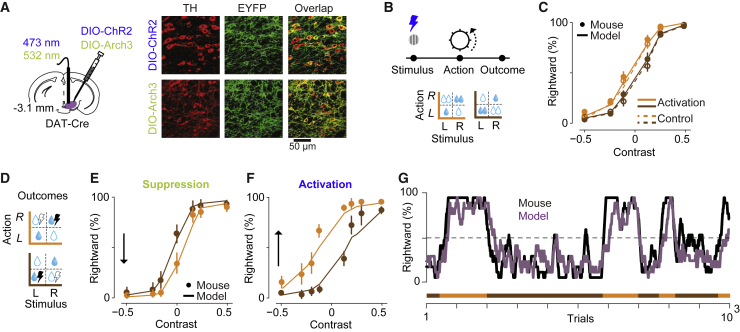
The experiments included sessions with blocks of trials with unequal water rewards and sessions with no reward size manipulation. In the optogenetic experiments, these sessions could include suppression of mPFC neurons or activation/suppression of VTA dopamine neurons. We fitted our model as well as reduced model variants on choices acquired in the task with unequal water rewards and cross-validated the necessity of model parameters. We then used the model that could best account for the data and fitted it on the experiments that included optogenetic manipulations. Experiments with unequal water reward For fitting, we set the value of smaller water reward to 1. Thus, the payoff matrix for blocks with larger reward on the left or right, respectively, are: o u t c o m e : [ 0 1 1 + x 0 ] , o u t c o m e : [ 0 1 + x 1 0 ] where x , a constant, represents the value of extra drop of water. We set the payoff for incorrect decisions to zero in all our model fitting. We fitted the model as well as reduced model variants on the decisions of mice in the task with unequal water rewards, and cross-validated the necessity of model parameters ( Figure S1 ). As described above, the full model included the following parameters: σ 2 , x , α . Each reduced model did not include one of these parameters. For σ 2 , one reduced model was set to have σ 2 = 0 , representing a model with no sensory noise, and the other reduced model was set to have σ 2 = ∞ , representing a model with extremely large sensory noise. For cross-validated fitting, we divided sessions of each mouse to 3 and performed a 3-fold cross validation. We performed the fit and parameter estimation on the training sessions and used the estimated parameters against the test sessions for computing goodness of fit. For fitting, we performed exhaustive search in the parameter space expanding large value range for each of the parameters to find the best set of model parameters that account for the observed decisions. We searched the following parameter space: α = 0 : 0.05 : 0.95 , σ 2 = 0.04 : 0.04 : 0.8 and x = − 5 : 0.2 : 10 . To do so, for each possible combination of these parameters, we repeatedly fed the sequences of stimuli that each mouse experienced to the model, observed decisions (iteration = 1000), and averaged across the iterations to compute the probability that model made a leftward and rightward decision ( P ˆ ( L ) , P ˆ ( R ) ) for each trial. We then calculated the negative log likelihood (NLL) as the average of – log ( P ˆ ( choice ) ) , where choice indicates the mouse’s decision in each trial ( Figure S1 ). The set of parameters that gave the lowest NLL were used to compute goodness of fit in the test sessions (3-fold cross-validation). Manipulation of mPFC activity For experiments including suppression of the mPFC at the stimulus onset, we allowed the model to add a constant to the predicted value of the choice Q C . A negative constant resulted in lower predicted value and hence increased prediction error after receiving a reward ( Figure S4 ). We fitted the model on choices as described above. The other possible way in which the model could be modified to show a larger shift in the psychometric curve is by simulating the effect of mPFC suppression as increasing the sensory noise ( σ 2 ) . However, this also results in curves with shallower slopes which we did not observe in the data ( Figure 4 ; Figure S4 ). Manipulation of dopamine activity For experiments including suppression or activation of dopamine neurons at the outcome time, we allowed the model to add a constant to the reward prediction error δ . This constant was negative for the experiment with dopamine suppression, and was positive for the experiment with dopamine activation ( Figure S5 ). We fitted the model on choices as described above.
Optimal observer model fitting
We constructed an alternative class of model that optimally performs our task. This observer leverages the structure of the task, i.e., it knows that only two reward sizes are available and that they switch side occasionally. The observer would thus only need to infer whether it is in the left or the right block, given the sequence of outcomes in the previous trials. To do so we used a hidden Markov model (MATLAB HMM toolbox). The model estimates the trial-by-trial probability that the current state is left or right block p ( S = L ) and p ( S = R ) , respectively, given a state transition matrix and an observation matrix. The state transition matrix defines the probability of block switch, which can be calculated from the number of block switches and number of trials in each dataset. The observation matrix defines the probability of observed outcomes (no reward, small reward and larger reward) given each state. The model computes the expected value of left and right actions according to: Q L = p L ( p ( S = L ) r ( a = L , s = L ) + p ( S = R ) r ( a = L , s = R ) ) and Q R = p R ( p ( S = L ) r ( a = R , s = L ) + p ( S = R ) r ( a = R , s = R ) ) , where p L and p R are estimated as described in the reinforcement learning model section, r ( a = L , s = L ) indicates the size of reward available for left action in the L block and p ( S = L ) and p ( S = R ) are the probabilities that the current trial belongs to L or R block, estimated using the hidden Markov model. This model learns about the blocks from any rewarded trials (both small and large rewards). This learning is, however, not influenced by the sensory confidence. When emission matrix is set optimally (i.e., in the left block the probability of large reward on the right is zero, p ( r = l a r g e | a = R , s = L ) = 0 , etc.), the model learns the block switch after only one rewarded trial. However, we observed that mice took several trials to learn the block switch ( Figure S1 ). Thus, for the fitting purpose, we considered that the observation matrix is noisy ( p ( r = l a r g e | a = R , s = L ) = β ) . An intuition behind this could be that the mouse does not always accurately detect the size of reward, and is hence slightly confused about the size of rewards which are available for L and R choices in each block; β determines this noise level. We estimated β for each animal using exhaustive search, as described in the previous section. After fitting, the model could account for the dependence of decisions on past rewards and current sensation ( Figure S1 ), but not for the dependence of choices on decision confidence in the previous trial ( Figure S1 ).
Additional behavioral analyses
The effect of sensory confidence on learning To isolate the effect of sensory confidence on learning ( Figures 1 E and 1F; Figures S1 E and S1F), we computed ‘Rightward (%)’ for each level of stimulus contrast conditional on preceding trial being a rewarded trial with either difficult or easy stimuli on the left or the right, resulting in four curves ( Figures 1 E and 1F). We then computed the difference between the two post-difficult curves and the difference between the two post-easy curves to compute Δ Rightward (%), as shown in Figure 1 E and Figure S1 E. This analysis involved an intermediate correction which ensures that the effect of past stimulus difficulty on choices is not due to slowly fluctuating bias over trials (i.e., serial correlation of choices due to slow side bias). This normalization procedure estimated the degree of choice bias in relation to possible bias in previous trials. We reasoned that slow fluctuations are, by definition, slower than one trial, and hence should be largely similar in adjacent trials. This assumption leads to a simple strategy to correct for possible drifts and isolate psychometric curve shifts due to past sensory confidence. To do so, we estimated ‘ Δ Rightward (%)’ conditional on preceding trial being a rewarded trial with either easy or difficult stimulus (as described above), and we also estimated ‘ Δ Rightward (%)’ conditional on the following trial being a rewarded one again with either easy or difficult stimulus. We then subtracted the latter from the former ( Figure 1 E; Figure S1 E). This removes the effect of slow response bias and provides an estimate of how the current trial influences choices in the next trial. Fitting of conventional psychometric function In order to test the effect of optogenetic manipulation on decisions, in addition to the model fitting described above, we used conventional psychometric fitting, Palamedes toolbox ( Prins and Kingdom, 2018 ), and tested whether the optogenetic manipulations influenced the slope and bias parameters of these fits. None of the manipulations influenced psychometric slopes, and the effect of manipulations on the bias was fully consistent with the results from our reinforcement model fittings. For analysis of reaction times, the reaction times from each session were first z-scored before averaging across sessions and animals.
Neuronal regression analysis
In order to quantify how each task event (stimulus, action, outcome) contributes to neuronal activity, and, the extent to which trial-by-trial variation in neuronal responses reflects animal’s estimate of pending reward and prediction error, we set up a neuronal response model ( Park et al., 2014 ) ( Figures 2 , 3 , S2 , and S3 ). We modeled the spiking activity of a neuron during trial j , which we denote R j ( t ) as R j ( t ) = S j K s ( t ) ∗ X j s ( t ) + A j K a ( t ) ∗ X j a ( t ) + O j K o ( t ) ∗ X j o ( t ) In the above equation, K s ( t ) , K a ( t ) and K o ( t ) are the profiles (kernels) representing the response to the visual stimulus, the action, and the outcome. X j s ( t ) , X j a ( t ) and X j o ( t ) are indicator functions which signify the time point at which the stimulus, action and outcome occurred during trial j . S j , A j and O j are multiplicative coefficients which scale the corresponding profile on each trial and ∗ represents convolution. Therefore, the model represents neuronal responses as the sum of the convolution of each task event with a profile corresponding to that event, which its size was scaled in each trial with a coefficient to optimally fit the observed response. Given the temporal variability of task events in different trials, the profile for a particular task event reflects isolated average neuronal response to that event with minimal influence from nearby events. The coefficients provide trial-by-trial estimates of neuronal activity for each neuron. The model was fit and cross-validated using an iterative procedure, where each iteration consisted of two steps. In the first step the coefficients S j , A j and O j were kept fixed and the profile shapes were fitted using linear regression. Profiles were fitted on 80% of trials and were then tested against the remaining 20% test trials (5-fold cross-validation). In the second step, the profiles were fixed and the coefficients that optimized the fit to experimental data were calculated, also using linear regression. Five iterations were performed. In the first iteration, the coefficients were initialized with value of 1. We applied the same analysis on the GCaMP responses ( Figure 3 ; Figure S3 ). We defined the duration of each profile to capture the neuronal responses prior to or after that event and selected longer profile durations for the GCaMP data to account for Ca +2 transients (mPFC spike data: stimulus profile: 0 to 0.6 s, action profile: −0.4 to 0.2 s, outcome profile: 0 to 0.6 s; GCaMP data: stimulus profile: 0 to 2 s, action profile: −1 to 0.2 s, outcome profile: 0 to 3 s, where in all cases 0 was the onset of the event). For both spiking and GCaMP data, the neuronal responses were averaged using a temporal window of 20 and 50 ms, respectively, and were then z-scored.
Data and Code Availability
The datasets supporting the current study have not been deposited in a public repository because of large file size, but are available from the corresponding author on request.
Lead Contact and Materials Availability
Further information and requests should be directed to and will be fulfilled by the Lead Contact, Armin Lak ( armin.lak@dpag.ox.ac.uk ). This study did not generate new unique reagents.
Experimental Model and Subject Details
The data presented here was collected from 33 mice (19 male) aged between 10-24 weeks. Wild-type C57/BL6J mice, DAT-Cre mice backcrossed with C57/BL6J mice (B6.SJLSlc6a3tm1.1(cre)Bkmn/J) and Pvalb-Cre mice backcrossed with C57/BL6J (B6.129P2-Pvalb tm1(cre)Arbr /J) were used. All experiments were conducted according to the UK Animals Scientific Procedures Act (1986) under appropriate project and personal licenses.
Method Details Surgeries
All mice were first implanted with a custom metal head plate. To do so, the animals were anesthetized with isoflurane, and were kept on a feedback-controlled heating pad (ATC2000, World Precision Instruments, Inc.). Hair overlying the skull was shaved and the skin and the muscles over the central part of the skull were removed. The skull was thoroughly washed with saline, followed by cleaning with sterile cortex buffer. The head plate was attached to the bone posterior to bregma using dental cement (Super-Bond C&B; Sun Medical). For electrophysiological experiments, we covered the exposed bone with Kwik-Cast (World Precision Instruments, Inc.), trained the animals in the behavioral task in the following weeks, and subsequently performed a craniotomy over the frontal cortex for lowering the silicon probes. For fiber photometry and optogenetic experiments, after the head plate fixation, we made a craniotomy over the target area (mPFC or VTA) and injected viral constructs followed by implantation of the optical fiber, which was secured to the head plate and skull using dental cement. Post-operative pain was prevented with Rimadyl on the three following days. Behavioral tasks Behavioral training started at least 7 days after the head plate implantation surgery. For mice which received viral injection, training started 2 weeks after the surgery. Animals were handled and acclimatized to head fixation for 3 days, and were then trained in a 2-alternative forced choice visual detection task ( Burgess et al., 2017 ). After the mouse kept the wheel still for at least 0.5 s, a sinusoidal grating stimulus of varying contrast appeared on either the left or right monitor, together with a brief tone (0.1 s, 12 kHz) indicating that the trial had started. The mouse could immediately report its decision by turning the wheel located underneath its forepaws. Wheel movements drove the stimulus on the monitor, and a reward was delivered if the stimulus reached the center of the middle monitor (a correct trial), but a 2 s white noise was played if the stimulus reached the center of the either left or right monitors (an error trial). The inter trial interval was set to 3 s. As previously reported, well-trained mice often reported their decisions using fast stereotypical wheel movements ( Burgess et al., 2017 ). In the initial days of the training (first 4 to 7 days), stimuli had contrast = 1. Lower-contrast stimuli were introduced when the animal reached the performance of ∼70%. After 2-3 weeks of training, the task typically included 7 levels of contrast (3 on the left, 3 on the right and zero contrast) which were presented in a random order across trials with equal probability. We finally introduced unequal water rewards for correct decisions: in consecutive blocks of 50-350 trials (drawn from a uniform distribution), correct decisions to one side (left or right) were rewarded with larger reward (2.4 μL versus 1.2 μL of water) ( Figure 1 ). Experiments involving optogenetic manipulation of mPFC neurons or VTA dopamine neurons had the same timeline as described above ( Figures 4 and 5 ). In experiments involving fiber photometry, the task timeline slightly differed from above, allowing longer temporal separation of stimulus, action and outcome ( Figure 3 ). In these experiments, wheel movements immediately after the visual stimulus did not move the stimulus on the monitor and did not result in a decision (open-loop condition). Instead, an auditory go cue (0.1 s) which was played 0.6-1.8 s after the stimulus onset started the closed-loop during which animals could report the decision. Wheel movements prior to go cue did not terminate the trial and we did not exclude these trials from our analysis (excluding these trials did not affect our results). In these experiments, we defined the action time as the onset of first wheel movement after the stimulus onset. In all experiments, reaction times were measured from the onset of visual stimulus till the onset of the first wheel movement. The behavioral experiments were controlled by custom-made software written in MATLAB (Mathworks) which is freely available ( Bhagat et al., 2019 ). Instructions for hardware assembly are also freely available ( https://www.ucl.ac.uk/cortexlab/tools/wheel ). Electrophysiological experiments We recorded neuronal activity in prelimbic region of mPFC using multi-shank silicon probes in wild-type C57/BL6J mice. We implanted the animals after they fully learned to perform the task, performing the final stage of the behavioral task (including block switches) with performance above 70% for at least three sessions. A 32-channel, 2 shank silicon probe (Cambridge NeuroTech) was mounted on a moveable miniature Microdrive (Cambridge NeuroTech) and implanted it into mPFC (n = 6 mice). On the implantation day, we removed the Kwik-Cast cover from the skull and drilled a small incision in the cranium over the frontal cortex, ML = 0.3 mm, AP = 1.8 mm (burr #19007–07, Fine Science Tools). The brain was protected with Ringer solution. We lowered the probe through the intact dura using a manipulator (PatchStar, Scientifica) to 1.4 mm from the dura surface. The final approach toward the target depth (the last 100–200 μm) was performed at a low speed (2–4 μm/sec), to minimize potential damage to brain tissue. Once the probe was in its required position, we waited 10 minutes to let the brain recover from the insertion and fixed the Microdrive on the head plate using dental cement. For reference signal we used a skull screw implanted on the skull ∼3-4 mm posterior to the recording site. At the end of each recording day we lowered the Microdrive 100 μm. Recordings were performed using OpenEphys system. Broadband activity was sampled at 30 kHz (band pass filtered between 1 Hz and 7.5 kHz by the amplifier) and stored for offline analysis. Recorded spikes were sorted with KlustaSuite ( Rossant et al., 2016 ). Manual spike sorting was performed oblivious to task-related responses of the units. Fiber photometry experiments To measure the activity of dopamine neurons, we employed fiber photometry ( Gunaydin et al., 2014 , Lerner et al., 2015 ). We injected 0.5 μL of diluted viral construct (AAV1.Syn.Flex.GCaMP6m.WPRE.SV40) into the VTA:SNc (ML:0.5 mm from midline, AP: −3 mm from bregma and DV:-4.4 mm from the dura) of DAT-Cre mice backcrossed with C57/BL6J mice (B6.SJLSlc6a3tm1.1(cre)Bkmn/J). We implanted an optical fiber (400 μm, Doric Lenses Inc.) over the VTA, with the tip 0.05 mm above the injection site. We used a single chronically implanted optical fiber to deliver excitation light and collect emitted fluorescence. We used multiple excitation wavelengths (465 and 405 nm) modulated at distinct carrier frequencies (214 and 530 Hz) to allow for ratiometric measurements. Light collection, filtering, and demodulation were performed as previously described ( Lerner et al., 2015 ) using Doric photometry setup and Doric Neuroscience Studio Software (Doric Lenses Inc.). For each behavioral session, least-squares linear fit was applied to the 405nm control signal, and the ΔF/F time series was then calculated as ((490nm signal – fitted 405nm signal) / fitted 405nm signal). All analyses were done by calculating z-scored ΔF/F. Optogenetic experiments Optogenetic manipulation of mPFC neurons For suppressing mPFC responses, we injected 0.5 μL of diluted viral construct containing ChR2 (AAV5.EF1a.DIO.hChr2(H134R)-eYFP.WPRE) unilaterally into the mPFC (ML:0.3 mm, AP: 1.8 mm from bregma and DV:-1.6 mm from the dura) of Pvalb-Cre mice backcrossed with C57/BL6J (B6.129P2-Pvalb tm1(cre)Arbr /J). We implanted an optical fiber (200 μm, Doric Lenses Inc.) over the mPFC, with its tip staying 0.4 mm above the injection site. We waited 2 weeks for virus expression and then started the behavioral training. After achieving stable task performance using symmetric water rewards, we introduced laser pulses which had following parameters: 473 nm (Laserglow LTD), number of pulses: 12, each pulse lasting 10 ms and separated by 30 ms, laser power: ∼2-3 mW (measured at the fiber tip). The laser pulses were applied either from the stimulus onset ( Figure 4 ; Figure S4 ) or during the outcome ( Figure S4 ). Manipulation at the time of the stimulus included three types of experiments: a) in 40% of randomly chosen trials in the task that had blocks of 50-350 trials with unequal rewards, b) in the task that had blocks of 50-350 trials with unequal rewards each of them with or without laser pulse at the stimulus time, making four types of blocks, c) in 40% of randomly chosen trials of a purely visual task (with symmetric and stable rewards). In the experiments involving manipulations at the trial outcome, in consecutive blocks of 50-350 trials, correct decisions to one side, L or R, were paired with laser pulses ( Figure S4 ).
Optogenetic manipulation of VTA dopamine neurons
For activating or suppressing dopamine neurons, We injected 0.5 μL of diluted viral constructs containing ChR2 (AAV5.EF1a.DIO.hChr2(H134R)-eYFP.WPRE) or Arch3 (rAAV5/EF1a-DIO-eArch3.0-eYFP) unilaterally into VTA:SNc (ML:0.5 mm from midline, AP: −3 mm from bregma and DV:-4.4 mm from the dura) of DAT-Cre mice backcrossed with C57/BL6J mice (B6.SJLSlc6a3tm1.1(cre)Bkmn/J). We implanted an optical fiber (200 μm, Doric Lenses Inc.) over the VTA, with its tip staying 0.4 mm above the injection site. We waited 2 weeks for virus expression and then started the behavioral training. After achieving stable task performance using symmetric water rewards, we introduced laser pulses which had the following parameters: 473 nm and 532 nm for ChR2 and Arch3, respectively (Laserglow LTD), number of pulses: 12, each pulse lasting 10 ms and separated by 30 ms, laser power: ∼8 mW (measured at the fiber tip). For the suppression experiment using Arch3, in few sessions we used a single 300 ms long pulse. The laser pulses were applied either 0.4 s prior to the stimulus ( Figure S5 ), exactly at the time of the stimulus ( Figure 5 ; Figure S5 ), or at the time of the reward ( Figure 5 ; Figure S5 ). For experiments involving activation of dopamine neurons prior to the stimulus onset, in 40% of randomly chosen trials, we delivered laser pulses. For experiments involving activation of dopamine neurons at the stimulus onset, we either applied pulses in 40% of randomly chosen trials ( Figure S5 ) or in blocks of 50-350 trials ( Figure 5 ). In the experiments involving manipulation of dopamine activity at the trial outcome, in consecutive blocks of 50-350 trials, correct decisions to one side, L or R, were paired with laser pulses ( Figure 5 ). In experiments involving trial-by-trial manipulations at the trial outcome (rather than blocks of trials), in 30% of randomly chosen correct trials, the reward was paired with laser pulses ( Figure S5 ). In both these experiments the laser was turned on simultaneously with the TTL signal that opened the water valve. Histology and anatomical verifications To verify expression of viral constructs we performed histological examination. Animals were deeply anesthetized and perfused, brains were post-fixed, and 60 μm coronal sections were collected. For optogenetic experiments on mPFC, we immunostained with antibody to eYFP and secondary antibodies labeled with Alexa Fluor 488 ( Figure 4 ). For experiments on dopamine neurons (both photometry and optogenetic), sections were immunostained with antibody to TH and secondary antibodies labeled with Alexa Fluor 594. For animals injected with ChR2 or Arch3 constructs into the VTA, we also immunostained with an antibody to eYFP and secondary antibodies labeled with Alexa Fluor 488 ( Figure 5 ; Figure S5 ). We confirmed viral expression in all animals with ChR2 injections into the mPFC and in 14 (out of 15) mice injected with ChR2, Arch3 or GCaMP6M. The anatomical location of implanted optical fibers was determined from the tip of the longest fiber track found, and matched with the corresponding Paxinos atlas slide ( Figures 3 , 4 , and 5 ; Figures S4 and S5 ). To determine the position of silicon probes in mPFC, coronal sections were stained for GFAP and matched to the corresponding Paxinos atlas ( Figure 2 A). Confocal images from the sections were obtained using Zeiss 880 Airyscan microscope.
Supplemental Information Document S1. Figures S1–S5 Document S2. Article plus Supplemental Information
📊 Figures
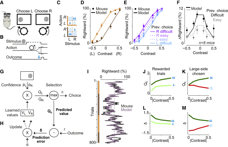
Figureu00a01
Behavioral and Computational Signatures of Decisions Guided by Reward Value and Sensory Confidence (A and B) Schematic of the 2-alternative visual task. After the mouse kept the wheel still for at lea...
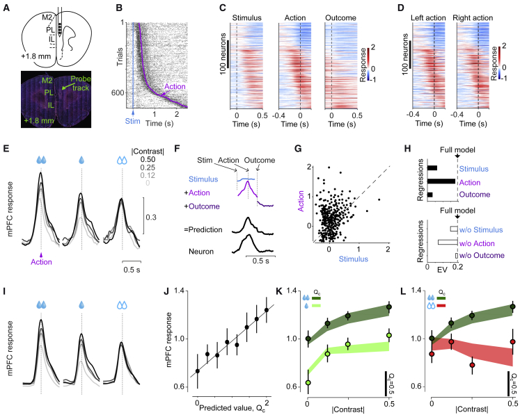
Figureu00a02
Medial Prefrontal Neurons Encode Confidence-Dependent Predicted Value (A) Histological image showing the high-density silicon probe track in mPFC. (B) Raster plot showing spikes of an example mPFC neu...
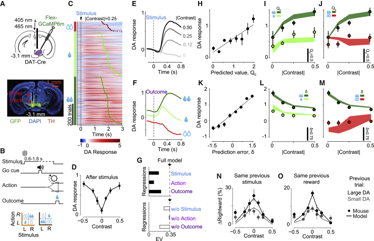
Figureu00a03
Dopamine Neurons Encode Confidence-Dependent Predicted Value and Prediction Error (A) Top: schematic of fiber photometry in VTA dopamine neurons. Bottom: example histology showing GCaMP expression and...
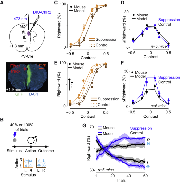
Figureu00a04
Learning Depends on Predicted Value Signaled by Medial Prefrontal Neurons (A) Top: to suppress mPFC population activity, we optogenetically activated Pvalb neurons by directing brief laser pulses thro...
Figureu00a05
Learning Depends on Prediction Error but Not Predicted Value Signaled by Dopamine Neurons (A) Left: ChR2 or Arch3 were expressed in dopamine neurons and a fiber implanted over VTA. Right: expression o...
Figure images are served from the NIH/NLM PubMed Central Open Access Subset or Europe PMC; copyright remains with the publishers and authors.
💬 Discussion
0 commentsNo comments yet. Be the first to start a discussion!
Leave a Comment