Abstract
The regulation of transcription requires the coordination of numerous activities on DNA, yet how transcription factors mediate these activities remains poorly understood. Here, we use lattice light-sheet microscopy to integrate single-molecule and high-speed 4D imaging in developing Drosophila embryos to study the nuclear organization and interactions of the key transcription factors Zelda and Bicoid. In contrast to previous studies suggesting stable, cooperative binding, we show that both factors interact with DNA with surprisingly high off-rates. We find that both factors form dynamic subnuclear hubs, and that Bicoid binding is enriched within Zelda hubs. Remarkably, these hubs are both short lived and interact only transiently with sites of active Bicoid-dependent transcription. Based on our observations, we hypothesize that, beyond simply forming bridges between DNA and the transcription machinery, transcription factors can organize other proteins into hubs that transiently drive multiple activities at their gene targets. Editorial note: This article has been through an editorial process in which the authors decide how to respond to the issues raised during peer review. The Reviewing Editor's assessment is that all the issues have been addressed (<xref ref-type="decision-letter" rid="SA1">see decision letter</xref>).
🔬 Techniques
🔭 Microscopes
🧬 Organisms
💻 Software
✨ Fluorophores
🧪 Sample Preparation
🏭 Microscope Brands
🧪 Reagent Suppliers
📷 Detectors
🔎 Objectives
🎨 Filters
💻 Software Details
💻 Code & Software
💾 Data Repositories
🏛️ Research Organizations (ROR)
Affiliated research institutions:
📋 Methods
Key resources table
Reagent type (species) or resource Designation Source or reference Identifiers Additional information Strain, strain background ( D. melanogaster ) mNeonGreen-Zld this paper Fly line with an N-terminal mNeonGreen fusion tag inserted at the endogenous Zld locus. Strain, strain background ( D. melanogaster ) mEos3.2-Zld this paper Fly line with an N-terminal mEos3.2 fusion tag inserted at the endogenous Zld locus. Strain, strain background ( D. melanogaster ) H2B-EGFP this paper Fly line with an H2B-EGFP transgene inserted on chromosome 3. Transgene is expressed ubiquitously under the control of a synthetic tubulin promoter. Strain, strain background ( D. melanogaster ) H2B-mEos3.2 this paper Fly line with an H2B-mEos3.2 transgene inserted on chromosome 3. Transgene is expressed ubiquitously under the control of a synthetic tubulin promoter. Strain, strain background ( D. melanogaster ) MCP-mcherry H Garcia lab Fly line with MCP-mCherry inserted as a transgene on chromosome 2. Genetic reagent ( D. melanogaster ) sgRNA #1 bicoid this paper sgRNA targeting N-terminus of Bcd gene, sequence GCGGAGTGTTTGGGGAAAA Genetic reagent ( D. melanogaster ) sgRNA #1 bicoid this paper sgRNA targeting N-terminus of Bcd gene, sequence TAAAAGTTTTGATCTGGCGG Genetic reagent ( D. melanogaster ) sgRNA #1 bicoid this paper sgRNA targeting N-terminus of Bcd gene, sequence TGATGGTAAAAGTTTTGATC Genetic reagent ( D. melanogaster ) sgRNA Zelda M Harrison lab sgRNA targeting N-terminus of Zld gene, sequence CCTCTGCCGCGTGCAGGGG Software, algorithm Spot-On Hansen et al., 2018 , eLife Generation of transgenic fly lines The following fly lines were constructed using CRISPR/Cas9 mutagenesis with homology directed repair: mNeonGreen-Zelda, mEos3.2-Zelda, mEos3.2-Bicoid. sgRNAs targeting sites near the desired insertion sites were cloned via the primer annealing method into plasmid pMRS-1, which is a version of pCFD3 ( Port et al., 2014 ) (addgene #49410) with alterations to the sgRNA body made according to ( Chen et al., 2013 ). sgRNA sequences were CCTCTGCCGCGTGCAGGGG for Zelda and an equimolar mixture of TGATGGTAAAAGTTTTGATC , GCGGAGTGTTTGGGGAAAA , and TAAAAGTTTTGATCTGGCGG for Bicoid. Homology directed repair templates were constructed in a pUC19 backbone via Gibson assembly with the desired tag, with an N-terminal FLAG tag, flanked by 1 kb homology arms. Fluorescent tags were inserted at the ATG located at 3R:6759268 for Bicoid and at X:19782283 for Zelda (dm6 coordinates). For both Zelda and Bicoid, the natural start ATG was removed, and the fluorescent protein and linker were fused with the first amino acid after the initiation Methionine residue. We tested a number of linker sequences and found variable tag- and protein-specific effects on viability. Linker sequences that yielded homozygous viable animals were GDGAGLIN (mNeonGreen-Zld), GGGGSGSGGS (mEos3.2-Zld and mEos3.2-Bcd) and GGGGSGSGGSMTRDYKDDDDKTRGS (H2B-mEos3.2 and H2B-EGFP). HDR template and sgRNA plasmids were sent to Rainbow Transgenic Flies, Inc. (Camarillo, CA) to be injected into embryos expressing Cas9 in the germline. Resulting adult flies were crossed to flies possessing balancer chromosomes matching the relevant chromosome. Single F1 progeny carrying the marked balancer were crossed to balancer stock flies, allowed 4–8 days for females to lay sufficient eggs, and the F1 parents were sacrificed for PCR genotyping. Typically, we find that ~ 10–40% of F1 animals contain insertions. For example, for a pooled injection of three Zelda tagging constructs, we screened 79 F1 animals and recovered 36 hits, of which we screened 19 to determine the identify of the inserted tag, recovering 8 GFP-Zld, 6 mEos3.2-Zld, and 5 HaloTag-Zld. We find that efficiency varies for different genes and injections, but these results are fairly typical. For positive hits, balanced lines were generated by selecting appropriately-marked F2 progeny, and F3 animals were examined for the presence of homozygous animals, revealed by the lack of balancer phenotype. As Bicoid has only maternal phenotypes, homozygous mothers were tested for the ability to give viable offspring. Lines that tolerated homozygous insertions were subjected to further screening by the preparation of clean genomic DNA, amplification of the locus using primers outside the donor homology arms, and subsequent Sanger sequencing of the entire amplicon. Lines carrying insertions free of mutations and containing no incorporated plasmid backbone were kept and utilized for imaging experiments. His2B-mEos3.2 was introduced as a supplemental transgene under the control of a ubiquitous pΔTubHA4C promoter ( Zhang et al., 2013 ) and SV40 3’ UTR via PhiC31-mediated recombinase ( Groth et al., 2004 ) into landing site VK33 ( Venken et al., 2009 ). A transgene was used to avoid potential complications associated with editing the highly multicopy histone locus. We chose a red fluorescent protein for single-molecule imaging in embryos as better signals are achievable at longer wavelengths. First, as is well known, there is high autofluorescence at greener wavelengths in the Drosophila embryo (and for most biological materials). Second, Rayleigh scattering, scattering from particles of sizes less than the wavelength of the imaging light (the phenomenon responsible for blue skies and red sunsets), scales as ~1/λ 4 where λ is the imaging wavelength. Thus, using longer wavelengths results in fewer photons being scattered and thus more photons being absorbed, emitted and collected from single molecules ( Mir et al., 2018 ).
Show full methods section
Key resources table
Reagent type (species) or resource Designation Source or reference Identifiers Additional information Strain, strain background ( D. melanogaster ) mNeonGreen-Zld this paper Fly line with an N-terminal mNeonGreen fusion tag inserted at the endogenous Zld locus. Strain, strain background ( D. melanogaster ) mEos3.2-Zld this paper Fly line with an N-terminal mEos3.2 fusion tag inserted at the endogenous Zld locus. Strain, strain background ( D. melanogaster ) H2B-EGFP this paper Fly line with an H2B-EGFP transgene inserted on chromosome 3. Transgene is expressed ubiquitously under the control of a synthetic tubulin promoter. Strain, strain background ( D. melanogaster ) H2B-mEos3.2 this paper Fly line with an H2B-mEos3.2 transgene inserted on chromosome 3. Transgene is expressed ubiquitously under the control of a synthetic tubulin promoter. Strain, strain background ( D. melanogaster ) MCP-mcherry H Garcia lab Fly line with MCP-mCherry inserted as a transgene on chromosome 2. Genetic reagent ( D. melanogaster ) sgRNA #1 bicoid this paper sgRNA targeting N-terminus of Bcd gene, sequence GCGGAGTGTTTGGGGAAAA Genetic reagent ( D. melanogaster ) sgRNA #1 bicoid this paper sgRNA targeting N-terminus of Bcd gene, sequence TAAAAGTTTTGATCTGGCGG Genetic reagent ( D. melanogaster ) sgRNA #1 bicoid this paper sgRNA targeting N-terminus of Bcd gene, sequence TGATGGTAAAAGTTTTGATC Genetic reagent ( D. melanogaster ) sgRNA Zelda M Harrison lab sgRNA targeting N-terminus of Zld gene, sequence CCTCTGCCGCGTGCAGGGG Software, algorithm Spot-On Hansen et al., 2018 , eLife Generation of transgenic fly lines The following fly lines were constructed using CRISPR/Cas9 mutagenesis with homology directed repair: mNeonGreen-Zelda, mEos3.2-Zelda, mEos3.2-Bicoid. sgRNAs targeting sites near the desired insertion sites were cloned via the primer annealing method into plasmid pMRS-1, which is a version of pCFD3 ( Port et al., 2014 ) (addgene #49410) with alterations to the sgRNA body made according to ( Chen et al., 2013 ). sgRNA sequences were CCTCTGCCGCGTGCAGGGG for Zelda and an equimolar mixture of TGATGGTAAAAGTTTTGATC , GCGGAGTGTTTGGGGAAAA , and TAAAAGTTTTGATCTGGCGG for Bicoid. Homology directed repair templates were constructed in a pUC19 backbone via Gibson assembly with the desired tag, with an N-terminal FLAG tag, flanked by 1 kb homology arms. Fluorescent tags were inserted at the ATG located at 3R:6759268 for Bicoid and at X:19782283 for Zelda (dm6 coordinates). For both Zelda and Bicoid, the natural start ATG was removed, and the fluorescent protein and linker were fused with the first amino acid after the initiation Methionine residue. We tested a number of linker sequences and found variable tag- and protein-specific effects on viability. Linker sequences that yielded homozygous viable animals were GDGAGLIN (mNeonGreen-Zld), GGGGSGSGGS (mEos3.2-Zld and mEos3.2-Bcd) and GGGGSGSGGSMTRDYKDDDDKTRGS (H2B-mEos3.2 and H2B-EGFP). HDR template and sgRNA plasmids were sent to Rainbow Transgenic Flies, Inc. (Camarillo, CA) to be injected into embryos expressing Cas9 in the germline. Resulting adult flies were crossed to flies possessing balancer chromosomes matching the relevant chromosome. Single F1 progeny carrying the marked balancer were crossed to balancer stock flies, allowed 4–8 days for females to lay sufficient eggs, and the F1 parents were sacrificed for PCR genotyping. Typically, we find that ~ 10–40% of F1 animals contain insertions. For example, for a pooled injection of three Zelda tagging constructs, we screened 79 F1 animals and recovered 36 hits, of which we screened 19 to determine the identify of the inserted tag, recovering 8 GFP-Zld, 6 mEos3.2-Zld, and 5 HaloTag-Zld. We find that efficiency varies for different genes and injections, but these results are fairly typical. For positive hits, balanced lines were generated by selecting appropriately-marked F2 progeny, and F3 animals were examined for the presence of homozygous animals, revealed by the lack of balancer phenotype. As Bicoid has only maternal phenotypes, homozygous mothers were tested for the ability to give viable offspring. Lines that tolerated homozygous insertions were subjected to further screening by the preparation of clean genomic DNA, amplification of the locus using primers outside the donor homology arms, and subsequent Sanger sequencing of the entire amplicon. Lines carrying insertions free of mutations and containing no incorporated plasmid backbone were kept and utilized for imaging experiments. His2B-mEos3.2 was introduced as a supplemental transgene under the control of a ubiquitous pΔTubHA4C promoter ( Zhang et al., 2013 ) and SV40 3’ UTR via PhiC31-mediated recombinase ( Groth et al., 2004 ) into landing site VK33 ( Venken et al., 2009 ). A transgene was used to avoid potential complications associated with editing the highly multicopy histone locus. We chose a red fluorescent protein for single-molecule imaging in embryos as better signals are achievable at longer wavelengths. First, as is well known, there is high autofluorescence at greener wavelengths in the Drosophila embryo (and for most biological materials). Second, Rayleigh scattering, scattering from particles of sizes less than the wavelength of the imaging light (the phenomenon responsible for blue skies and red sunsets), scales as ~1/λ 4 where λ is the imaging wavelength. Thus, using longer wavelengths results in fewer photons being scattered and thus more photons being absorbed, emitted and collected from single molecules ( Mir et al., 2018 ).
Western blot
For each genotype indicated, 50–60 embryos aged 2 hr at 25° were dechorionated in bleach, rinsed in salt solution (NaCl with TritonX-100) and flash frozen. Frozen embryos were homogenized in 50 µL of sample buffer and 20 µL of sample per lane was loaded onto two separate 4–15% SDS-PAGE gels (Bio-Rad Cat # 4561083DC). Western blots were performed using rabbit polyclonal α-Bcd or α-Zld primary antibodies and a goat α-rabbit HRP conjugated secondary antibody (Thermo Fisher Cat # 31460). MS2 crosses For MS2 experiments, yw; +; MCP-mCherry (gift from S. Alamos and H.G. Garcia) virgin females were crossed to males homozygous for either EGFP-Bcd or mNeonGreen-Zld. Resulting female progeny maternally deposit both MCP and the labeled TF in embryos. Virgin females were crossed to males homozygous for the hb MS2 BAC and resulting embryos were used for imaging.
Lattice light-sheet microscopy of live embryos
Embryos were collected from flies in small cages over a 90-min laying period. Prior to embryo collection, the surface of a 5 mm diameter glass coverslip was made adhesive by deposition of of a small drop of glue solution (the glue solution was prepared by dissolving a roll of double-sided scotch tape in heptane overnight). The coverslip was allowed to dry for at least 5 min, which is sufficient time for the heptane to evaporate leaving behind a sticky surface. Embryos were washed off from the cage lids using tap water and gentle agitation with a paintbrush into a nylon cell-strainer basket. Embryos were then dechorionated in 100% bleach for 90 s. The dechorionation was then stopped by continuous washing under tap water until no further bleach smell could be detected, typically 30 s. The embryos were then transferred from the water filled strainer basket onto an agar pad using a fine haired paintbrush and arranged into an array of typically 3 rows and five columns with a consistent anteroposterior (A-P) orientation. The arranged embryos were then gently contact transferred onto the adhesive coverslip which was subsequently loaded into the microscope sample holder. A home built lattice light-sheet microscope (LLSM) was used ( Chen et al., 2014a ; Chen et al., 2014b ; Mir et al., 2017 ) for all single molecule, bulk fluorescence, and MS2 imaging experiments. Images were acquired using two Hamamatsu ORCA-Flash 4.0 digital CMOS cameras (C13440-20CU). An image splitting long-pass dichroic (Semrock FF-560) was placed in between the two cameras to separate emission wavelengths of over and under 560 nm, in addition bandpass filters corresponding to the fluorophore of interest were installed in front of each camera to provide further spectral filtering (Semrock FF01-525/50 for mNeon and sfGFP, Semrock FF01-593/46 for mEOS3.2, and Semrock FF01-629/53 for mCherry). Further details of imaging settings and conditions for each type of imaging experiment are provided in the corresponding sections below. For all experiments, the stage positions corresponding to the anterior and posterior extents of each embryo imaged were recorded. The position along the anteroposterior axis for each image or movie recorded was then calculated as a fraction of the embryonic length (EL) with 0 and 1 to the anterior and posterior extents of the embryo, respectively. The nuclear cycle and progression within the nuclear cycle (e.g. interphase, prophase, mitosis) were also recorded for each movie or image. Times between nuclear cycles were also monitored to ensure that data was being acquired on a healthy and normally developing embryos. Embryos which exhibited aberrant development, for example longer than usual nuclear cycles, or numerous aberrant nuclear divisions were abandoned and the data was discarded.
Single-molecule imaging and tracking in live embryos
For single-molecule imaging experiments, the illumination module of the LLSM was modified to provide constant photoactivation using a 405 nm laser line that bypasses the Acousto-optical tunable filter (AOTF) ( Figure 1—figure supplement 1 ). We found that even when a lattice pattern for 561 nm was displayed on the spatial light modulator (SLM) sufficient 405 nm illumination was present in the imaging plane to allow for controlled photo-activation of mEos3.2-Bcd and mEos3.2-Zld. For all single-molecule experiments, a 30 beam square lattice with 0.55 and 0.44 inner and outer Numerical Apertures, respectively, was used in dithered mode for excitation. The 405 nm laser line was kept on constantly during the acquisition period for photoswitching and a 561 nm laser line was used for excitation. For both mEos3.2-Bcd and mEos3.2-Zld, data was acquired at 7.5, 100 and 500 ms exposure times with effective frame rates of 100, 9.52, and 1.98 Hz, respectively. The excitation laser power was optimized empirically for each exposure time to achieve sufficient contrast for single-molecule tracking and the powers of the photoswitching laser were also optimized empirically to achieve low enough densities of detections to enable tracking. The excitation laser power was 0.1 mW, 0.6 mW, 2.3 mW and switching laser power was 2.3 µW, 3.9 µW, and 8.5 µW for 500, 100, and 7.5 ms exposures, respectively, as measured at the back focal plane of the excitation objective. The same settings were used to acquire control data at each exposure time on His2B-mEos3.2. For all exposure times, the length of each acquisition was 105 s, corresponding to 200, 1000, and 10,000 frames at 500, 100, and 7.5 ms exposure times, respectively. The acquisition length was set so that sufficient fields of views could be captured in the short interphase times of the early nuclear cycles while also capturing a sufficient number of single-molecule trajectories. For characterization of single-molecule dynamics at these multiple time scales, both mEos3.2-Bcd and mEos3.2-Zld were measured in a His2B-EGFP background. The His2B-EGFP channel was used to ensure optimal positioning of the sample within the light-sheet, to keep track of progression through a cell cycle, and monitor the development of the embryo. A fortunate bonus was that at 100 ms and 500 ms exposures, there was sufficient excitation of His2B-EGFP from the photoactivation 405 nm laser that we could perform simultaneous imaging of chromatin and single-molecule dynamics ( Figure 1—video 3 and Figure 1—video 4 ). For quantification of single-molecule mEos3.2-Bcd dynamics in the context of mNeonGreen-Zld, single-molecule data was acquired for 1 s (10 frames at 100 ms exposure times), followed by 10 frames of acquisition in the mNeon channel at 10 ms exposure times, and this sequence was then repeated 100 times. The sum of the 10 mNeonGreen images was then calculated to effectively provide a 100 ms exposure image. This scheme was designed such that the dynamic motion of Zld could be captured in addition to the binding kinetics of Bcd with sufficient temporal resolution without having to modify the LLSM control software. The rest of the imaging parameters were kept identical to those described above. For all single-molecule experiments, nuclei from at least three embryos were measured spanning a range of anteroposterior positions and at nuclear cycles ranging from 12 to 14. Localization and tracking of single molecules was performed using a MATLAB implementation of the dynamic multiple-target tracing algorithm ( Sergé et al., 2008 ) as previously described ( Mir et al., 2017 ; Hansen et al., 2018 ; Hansen et al., 2017 ; Teves et al., 2016 ). Mean square displacement analysis Mean Square Displacement curves were calculated using the open source msdanalyzer package ( Tarantino et al., 2014 ). For analysis of sub-diffusive motion MSD/τ curves for His2B, Zld, and BCD plotted on log-log-scale. As for anomalous diffusion MSD(τ)=Γτ α , where α is the confinement factor the log(MSD/τ)=log(Γ) + (α−1)τ ( Izeddin et al., 2014 ). The log of the MSD/τ was thus used to estimate the range of α values for each protein. Analysis of short exposure (10 ms) single-molecule trajectories Single-molecule trajectories were analyzed using Spot-on ( Hansen et al., 2018 ), a freely available open-source software ( https://gitlab.com/tjian-darzacq-lab/spot-on-matlab ) based on a model previously introduced in Mazza et al. (2012) and modfied in Hansen et al. (2017) to exclude state transitions. In brief, Spot-On performs fits to the distribution of displacements at multiple frameshifts to a two-state kinetic model and provides estimates of the fraction of molecules bound and free, and the corresponding apparent diffusion coefficients for each state ( Figure 3—figure supplement 1 ) and corrects for the probability of molecules diffusing out of the axial detection range. We performed fitting using the following parameters: Gaps Allowed: 1, Jumps to Consider: 4, TimePoints: 8, Observation Slice: 0.8 μm, Fit Iterations 5. The fit parameters for each data set are summarized in Figure 3—figure supplement 1 . Data are represented as the mean over the three embryo replicates ±SEM.
Calculation of residence times from long exposure single-molecule trajectories
Imaging with sufficiently long exposure times effectively blurs out fast-moving molecules into the background while molecules stably bound for a significant duration of the exposure time are imaged as diffraction limited spots ( Hansen et al., 2017 ; Watanabe and Mitchison, 2002 ; Mir et al., 2017 ; Teves et al., 2016 ; Chen et al., 2014a ; Chen et al., 2014b ). Thus, the trajectories from the 500 ms datasets are used to infer the genome average long-lived (specific) binding times. To infer the residence time, the length of trajectories in time is used to calculate a survival probability (SP) curve (1- cumulative distribution function of trajectory lengths). Since the SP curve contains contributions from non-specific interactions, slowly moving molecules, and localization errors a double-exponential function of the form SP(t)=F*(exp(-k ns *t))+(1 F)(exp(-k s *t))is fit to the SP curve, where k ns is the off-rate for the short-lived (non-specific) interactions and k s correspond to the off-rate of long lived (specific) interactions ( Chen et al., 2014a ; Chen et al., 2014b ; Hansen et al., 2017 ; Mir et al., 2017 ) ( Figure 4—figure supplement 2 ). For fitting purposes, probabilities below 10 −3 are not used to avoid fitting the data poor tails of the distribution. An objective threshold on the minimum number of frames a trajectory lasts is then used to further filter out tracking errors and slow-diffusing molecules ( Mazza et al., 2012 ; Hansen et al., 2017 ). The objective threshold is determined by plotting the inferred slow rate constant and determining where values converge to a single value. Although the 500 ms Bcd data set converges at two frames (1 s), the Zld data set converges at four frames (2 s) ( Figure 4—figure supplement 2B–C ). The survival probability distribution for Zelda is likely dominated by short-lived interactions at shorter timescales and is most likely a reflection of the same complex mixed population (specific and non-specific DNA binding, along with another population whose motion is constrained perhaps by protein-protein interactions) we observed in the MSD curves ( Figure 2B ). Thus, a four-frame threshold was used for the calculation of the specific residence time. Next, since the inferred k s as described above is biased by photobleaching, and nuclear and chromatin movement, bias correction is performed using the His2B data as k s,true =k s -k bias , where k bias is the slower rate from the double-exponent fit to the His2B SP curve as described previously ( Teves et al., 2016 ; Hansen et al., 2017 ; Chen et al., 2014a ; Chen et al., 2014b ). This correction is based on the assumption that photobleaching, unbinding, and loss of trajectories from motion are all independent Poisson processes. The genome wide specific residence time is then calculated as 1/k s,true . The effectiveness of this bias correction is checked by calculating the residence time from both the 100 ms and 500 ms frame rate data and observing convergence to within 1 s ( Figure 4—figure supplement 2C ).
Fluorescence recovery after photobleaching
FRAP was performed on a Zeiss (Germany) LSM 800 scanning confocal microscope equipped with several laser lines, of which the 488 nm laser was used for all experiments described here. Images were collected using a Plan-Apochromat 63 × 1.40 NA oil-immersion objective using a window 50.7 µm by 3.6 µm. Bleaching was controlled by the Zen software, and experiments consisted of 10 frames collected before the bleach and 1000 frames collected after at a frame rate of 24 ms. In each frame, five circular bleach spots of 1 µm diameter were chosen to be a sufficient distance from nuclear edges. The spots were bleached using maximum laser intensity, with dwell time adjusted to 0.57 µs, which was chosen because it gave a sufficiently deep bleach of Bicoid, the fastest-recovering molecule we studied. Total bleach time was 1.5 s. We collected data from at least three embryos for each molecule studied. Nuclei in the early embryo are highly mobile, and we found that the most reliable method to find stable nuclei was to simply collect many movies and select the ones in which nuclei remain stable for the duration of the experiment. We collected movies with stable nuclei for a total of at least 50 bleach spots (50 nuclei) total for each molecule. To quantify and bleach-correct FRAP data, we used a custom-written MATLAB software pipeline ( Mir and Stadler, 2018 ; copy archived at https://github.com/elifesciences-publications/MirStadler_2018 ). Briefly, for each frame we manually select several ‘dark’ spots that are not within nuclei and several ‘control’ spots that are within bleached nuclei but well-separated from the bleach spot. We use a 600 nm diameter circle to calculate the signal at the spots in order to make the measurement robust to small chromatin movements. For each frame, the mean of the dark spots was subtracted from the bleach spot values (background subtraction), and individual bleach spot values were divided by the mean of the control spots to correct for the reduction in total nuclear fluorescence. Finally, the values for each spot were normalized to its mean value for the ten pre-bleach frames. We observed that chromatin movement occasionally causes the bleach spot to drift far enough to affect the signal, so we manually curated resulting correct traces to remove anomalous spots. This culling resulted in 27–40 quality recovery curves for each molecule. These curves were averaged for each molecule, and the mean recovery curve was used in figures and fitting. We fit resulting FRAP curves to the reaction-dominant model ( Sprague et al., 2004 ): FRAP(t) =1 - A e-k at - Be -kbt From these fits, we used the slower coefficient to estimate the time to half-recovery for the population of bound molecules.
Analysis of single-molecule binding in the context of Zld density
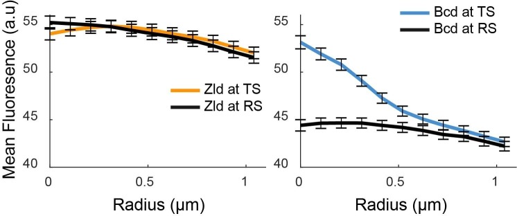
To analyze single-molecule trajectories of Bcd and Zld in the context of Zld density first, a relative density map for each nucleus was calculated. For each reconstructed 100 ms exposure Zld image, first each nucleus was identified and segmented out of the image using an in house segmentation algorithm built in MATLAB ( Figure 6—figure supplement 1 ). First, the grayscale image was Gaussian filtered with a sigma of 5 pixels to enhance the contrast of the nuclei, the filtered image was then thresholded using the inbuilt adaptive threshold function in MATLAB with a sensitivity value set to 0.6. A morphological dilation was then performed on the binary mask using a disk structuring element with a radius of 3 pixels and multiplied with hand drawn mask to remove edges of the embryo and non-cortical regions deep where no nuclei were present or imaging contrast was low. Holes within the nuclei binary mask were then filled using the MATLAB imfill function. A label matrix was generated from the resulting binary mask and the size distributions and eccentricities of segmented regions were calculated, an area and eccentricity cutoff was then applied to remove false positives to generate the final label matrix. Label matrices were then further curated to remove false positives. A relative density map was calculated for each nucleus individually by assigning each pixel in the nuclear value the percentile range it fell in over the entire distribution of intensity values in the nuclear area in with a resolution of 1 percentile. Each single-molecule trajectory was then assigned a relative density value based on the mean density of the pixels it fell in during the course of the trajectory. From visual examination, we determined that a 85 relative density value threshold was reliable in differentiating the highest enriched Zld regions, corresponding to hubs, from the rest of the nucleus. Fold change in densities of detections were calculated by counting the total number of trajectories in areas of relative density greater than 85 vs. the rest of the nucleoplasm. As the single-molecule trajectories from this data set are limited in length to 1 s, an accurate estimate of the residence time from fits to the survival probability distribution could not be obtained as was done above. Analysis of protein distribution in context of transcription dynamics Two-color 4D LLSM imaging was performed on embryos with the MS2-tagged hb BAC ( Figure 7—figure supplement 1 ) and expresing MCP-mCherry crossed with either mNeonGreen-Zld or eGFP-Bcd embryos. Z-stacks of 61 slices were acquired with a spacing of 250 nanometers to cover a range of 15 µm with an exposure time of 80–100 ms in each channel at each slice. Images in both channels were acquired at each z-position sequentially before moving to the next slice. The time between each volume acquired was ~5 s, the total length of the acquisition varied but at least one complete nuclear cycle was imaged for each embryo. The field of view for each embryo was centered at between 25% and 35% of the embryonic length from the anterior tip of the embryo to ensure that all nuclei in the image were within the hunchback expression domain. Data from a total of six embryos each for mNeonGreen-Zld or eGFP-Bcd were analyzed. To analyze the distribution of Zld or Bcd around sites of active hb transcription the signal from the MS2 site was used as a marker for the active locus. Each MS2 site was localized through a custom built detection software ( Figure 7—figure supplement 1 ). First, the data was manually examined and annotated to simplify the segmentation procedure by only considering frames in which transcription was occuring. A 3D difference of gaussian image was then calculated at each frame to enhance the contrast of the MS2 site, a global threshold was then applied to generate a 3D binary mask for each frame. The binary mask was filtered to remove structures too big or too small to be from a MS2 site and a label matrix was generated. The xyz weighted center of each labeled region was then used to calculate line profiles extended one micron from the center of the region in each direction. The ratio of the maximum and minimum values in the line profile were used to determine if the labeled region was in a nucleus. This calculation is effective as in the MCP-mCherry channel the nucleoplasm around the MS2 site appears dark whereas in the remainder of the embryo the background is high, thus labeled regions with low-contrast ratios were discarded. The maximum value of the profile of the remaining labeled regions was then used to localize the center of the active locus. The detected loci in each frame were then connected in time using a nearest neighbor algorithm. The position list of the detected and tracked active loci were then used to crop a 2.18 µm window around the center of each locus in x-y, if any part of the window did not lie within a nucleus the locus was not considered for further analysis. For the remaining loci, a control window was cropped at a distance of 2.6 µm from the center of the locus in x-y. If a control window could not be found that did not completely lie within the nucleus the corresponding locus was also not considered for further analysis. In this manner a total of 3943 and 6307 windows centered around loci and corresponding control points were accumulated from the Bcd and Zld datasets, respectively. The mean image at the locus was then calculated ( Figure 7C , Figure 7—video 4 , Figure 7—video 5 ) and a radial profile was calculated for Zld or Bcd centered at the active locus or the random control site. The radial profiles were then normalized to one at the maximum radius.
Additional files 10.7554/eLife.40497.038 Transparent reporting form Data availability All data generated or analysed during this study are included in the manuscript and supporting files. Source videos are also available on http://eisenlab.org/hubs and software through GitHub ( https://github.com/meisenlab/MirStadler_2018 ; copy archived at https://github.com/elifesciences-publications/MirStadler_2018 ).
📊 Figures
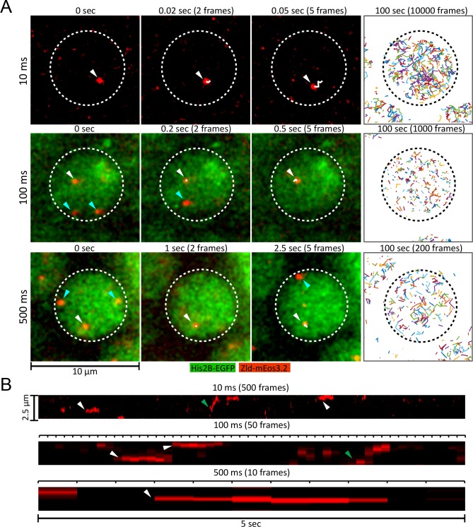
Figure 1.
Live embryo single-molecule imaging and tracking of endogenous mEos3.2-Zld.
( A ) First three columns are example images showing single molecules of mEos3.2-Zld tracked over at least five frames (white arrows and trajectories) at frame rates of 10, 100 and 500 ms.u00a0Cyan ar...
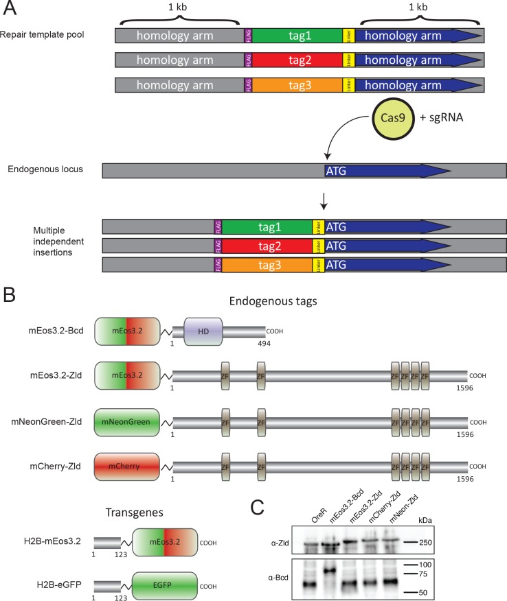
Figure 1u2014figure supplement 1.
Overview of CRISPR-Cas9 genome editing strategy.
( A ) Pools of homology repair template plasmids containing different protein tags were co-injected with a plasmid encoding an sgRNA targeting the N-terminus of the target coding sequence into embryos...
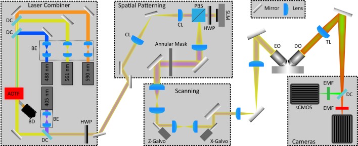
Figure 1u2014figure supplement 2.
Simplified Schematic of Lattice Light Sheet Microscope.
The schematic is organized to show the major modules of the microscope. The Laser Combiner module contains six lasers (three shown here) for excitation ranging from 405 to 639 nm, each of which are in...
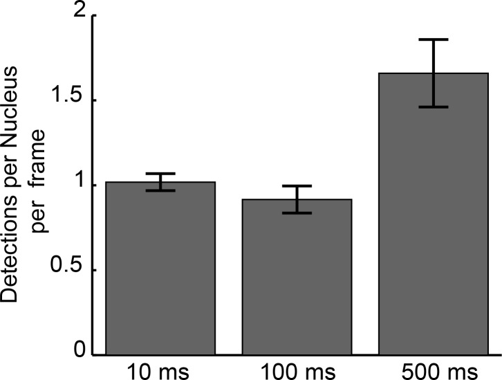
Figure 1u2014figure supplement 3.
Mean detections per nucleus per frame for each frame rate.
Detections per nucleus/frame characterized over 804245, 78281, 15165 frames of imaging and 169, 434, and 359 nuclei for 10 ms, 100 ms, and 500 ms, datasets respectively. Error bars show standard error...
Figure 1u2014videou00a01.
Movie illustrating ability to controllably photactiviate mEOS3.2.
Related to Figure 1 .u00a0Movie illustrating the ability to photo-activate mEos3.2 with the modified LLSM system. The power of the 405 nm laser was set to its highest value at approximately the 4 s ma...
Figure 1u2014videou00a02.
Example movie of mEos3.2-Zld acquired at 10 ms frame rate.
Related to Figure 1 .u00a0White scale bar is 5 u03bcm, images were gaussian filtered and inverted for display.
Figure 1u2014videou00a03.
Example movie of mEos3.2-Zld (red) and His2B-EGFP (green) acquired at 100 ms frame rate.
Related to Figure 1 .u00a0White scale bar is 5 u03bcm, a nucleus undergoing division is shown for illustrative purposes, data from mitotic nuclei were not used for single-molecule analysis in this wor...
Figure 1u2014videou00a04.
Example movie of mEos3.2-Zld (red) and His2B-EGFP (green) acquired at 500 ms frame rate.
Related to Figure 1 .u00a0White scale bar is 5 u03bcm, data from mitotic nuclei were not used for single-molecule analysis in this work. Images were gaussian filtered for display.
Figure 1u2014videou00a05.
Example of a mobile molecule of mEos3.2-Zld tracked at 10 ms frame rate.
Related to Figure 1 .u00a0White scale bar is 2 u03bcm. Images were gaussian filtered and inverted for display.
Figure 1u2014videou00a06.
Example of a immobile molecule of mEos3.2-Zld tracked at 10 ms frame rate.
Related to Figure 1 .u00a0White scale bar is 2 u03bcm. Images were gaussian filtered and inverted for display.
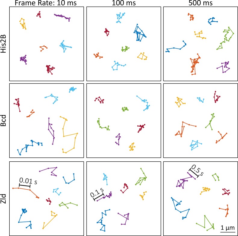
Figure 2.
Representative single-molecule trajectories of His2B, Bcd and Zelda.
Representative single-molecule trajectories of His2B, Bcd, and Zld from data acquired at frame rates of 10, 100 and 500 ms.
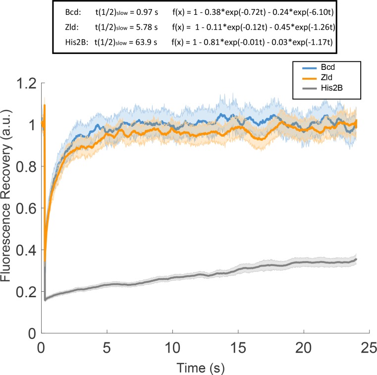
Figure 2u2014figure supplement 1.
Fluorescence recovery after photobleachingu00a0(FRAP).
FRAP curves for Bcd, Zld, and His2B and results of 2 exponential fitting. Solid lines are averages over at least 27 measurements and shaded regions indicate standard error.
Figure 2u2014videou00a01.
Comparison of single-molecule movies for His2B-mEos3.2, mEos3.2-Bcd, and mEos3.2-Zld at 10 ms frame rate.
Related to Figure 2 .u00a0White scale bar is 2 u03bcm. Panels left to right are His2B-mEos3.2, mEos3.2-Bcd, and mEos3.2-Zld. Images were gaussian filtered, inverted, and contrast was manually adjusted...
Figure 2u2014videou00a02.
Comparison of single-molecule movies for His2B-mEos3.2, mEos3.2-Bcd, and mEos3.2-Zld at 100 ms frame rate.
Related to Figure 2 .u00a0White scale bar is 2 u03bcm. Panels left to right are His2B-mEos3.2, mEos3.2-Bcd, and mEos3.2-Zld. Images were gaussian filtered, inverted, and contrast was manually adjusted...
Figure 2u2014videou00a03.
Comparison of single-molecule movies for His2B-mEos3.2, mEos3.2-Bcd, and mEos3.2-Zld at 500 ms frame rate.
Related to Figure 2 .u00a0White scale bar is 2 u03bcm. Panels left to right are His2B-mEos3.2, mEos3.2-Bcd, and mEos3.2-Zld. Images were gaussian filtered, inverted, and contrast was manually adjusted...
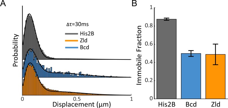
Figure 3.
Immobile Fraction of His2B, Zld, and Bcd molecules.
( A ) Histograms of displacements for His2B, Zld, and Bcd after three consecutive frames (u0394u03c4u00a0=u00a030 ms) at a frame rate of 10 ms.u00a0The Zld and Bcd distributions show a right tail indi...
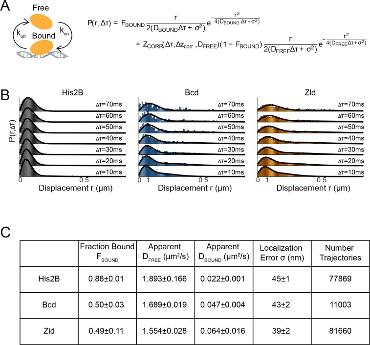
Figure 3u2014figure supplement 1.
Kinetic modeling of fast SPT data.
( A ) Overview of two-state model in which molecules are either in a free or bound state and the kinetic-model used to fit the displacement distributions, P(r,u0394u03c4), where F BOUND is the fractio...
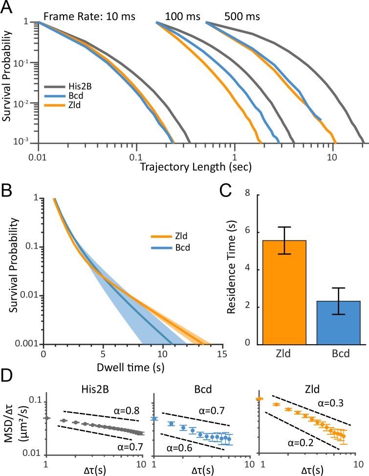
Figure 4.
Residence times and dynamics of bound Zld and Bcd molecules.
( A ) Raw survival probabilities of trajectories at all frame rates.u00a0Calculated over 77869, 81660, 11003, at 10 ms, 107998, 42698, 8990 at 100 ms, and 2420, 14487, 47681 at 500 ms, trajectories fo...
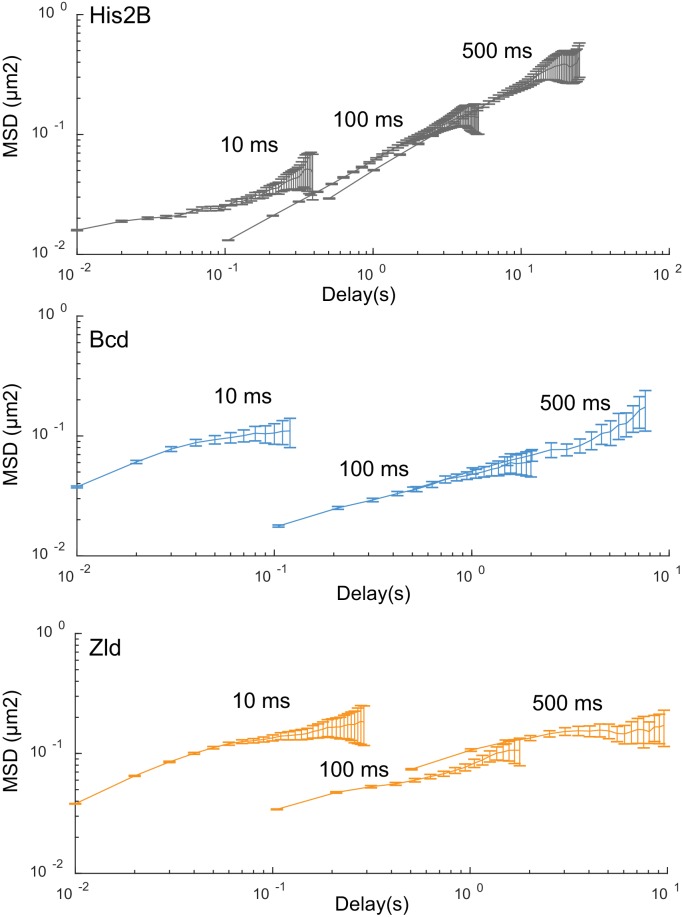
Figure 4u2014figure supplement 1.
Mean square displacement curves.
MSD curves for His2B, Zld, and BCD, at all frame rates plotted on log-log-scale.u00a0Calculated over 77869, 81660, 11003, at 10 ms, 107998, 42698, 8990 at 100 ms, and 2420, 14487, 47681 at 500 ms, tra...
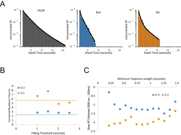
Figure 4u2014figure supplement 2.
Inference of residence times from single-molecule trajectories.
( A ) Example fits of two-exponent model (black line) to the survival probability (SP) distributions data from a single embryo for each protein studied ( B ) Bias corrected residence time (RT) as a fu...
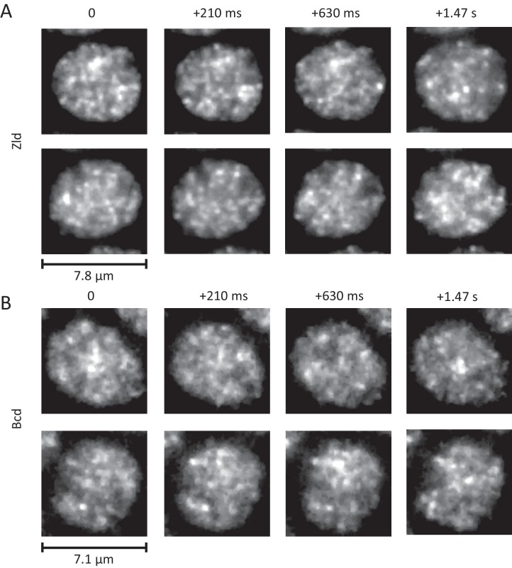
Figure 5.
Dynamic interphase hubs of Zld and Bcd.
Example images of the spatial distributions of Zld ( A ) and Bcd ( B ) at various time intervals illustrating the dynamic nature and wide range of size distributions and temporal persistences of enric...
Figure 5u2014videou00a01.
Cell cycle dynamics of Zelda spatial distribution.
Related to Figure 5 . Maximum intensity projection over 81 slices spaced at 250 nm apart. Right isu00a0His2B-mCherryu00a0and leftu00a0is sfGFP-Zld imaged through nuclear cycles 13 and 14. His2B is pre...
Figure 5u2014videou00a02.
Four-dimensional Interphase dynamics of Zld spatial distributions.
Related to Figure 5 .u00a0Three-dimensional rendering of Zld spatial distribution in nuclear cycle 13. Progress bar indicates time in minutes. Slice spacing in z is 200 nm, time between volumes is 9.5...
Figure 5u2014videou00a03.
Interphase dynamics of Zld spatial distributions at high temporal resolution.
Related to Figure 5 .u00a0Interphase dynamics of Zld spatial distribution at 10 ms exposure times and 15 ms frame rate.
Figure 5u2014videou00a04.
Four dimensional dynamics of Bcd spatial distribution.
Related to Figure 5 .u00a0Three-dimensional rendering of Bcd spatial distribution from nuclear cycles 13u201314. Progress bar indicates time in minutes. Slice spacing in z is 200 nm, time between volu...
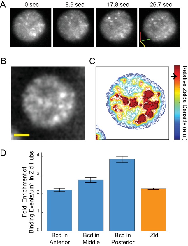
Figure 6.
Enrichment of Bcd binding in Zld hubs.
( A ) Three-dimensional volume renderings of an interphase nucleus showing the dynamic nature of Zld hubs (see Figure 5u2014video 2 , Figure 5u2014video 3 ).The 3D axes indicate the xyz axes and the a...
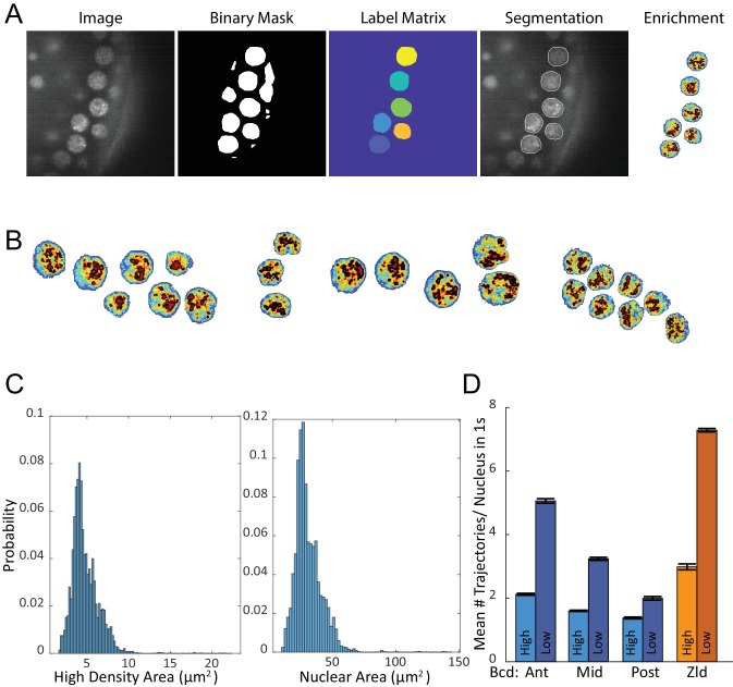
Figure 6u2014figure supplement 1.
Analysis of Zelda density.
( A ) Major steps in nuclear segmentation algorithm, the Zelda image is first low-pass filtered and then converted to a binary mask through adaptive thresholding, a hand drawn mask is applied to remov...
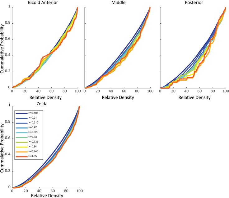
Figure 6u2014figure supplement 2.
Cumulative probability of trajectories vs. relative Zelda density.
Plots show the cumulative probability of a trajectory greater than oru00a0equal to a certain lengthu00a0inu00a0time (as indicated by color) vs. the relative density of Zld. The top row shows the proba...
Figure 6u2014videou00a01.
Bcd single-molecule localizations in context of the bulk spatial distribution of Zld.
Related to Figure 6 .u00a0Bicoid detections (red dots) overlaid on Zld spatial distribution. Each frame in the movie corresponds to 1 s of detections at 100 ms exposure times. Field of view is 9 u00d7...
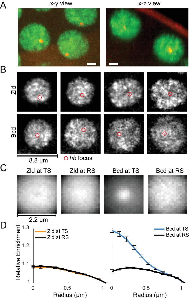
Figure 7.
Spatio-temporal distribution of Zld and Bcd hubs in context of active hb loci.
( A ) Representative x-y and x-z max projections over a nuclear diameter of mNeonGreen-Zld (green) and an active hb locus tagged with MS2-MCP-mCherry (red) white scale bars are 2 u03bcm. ( B ) Represe...
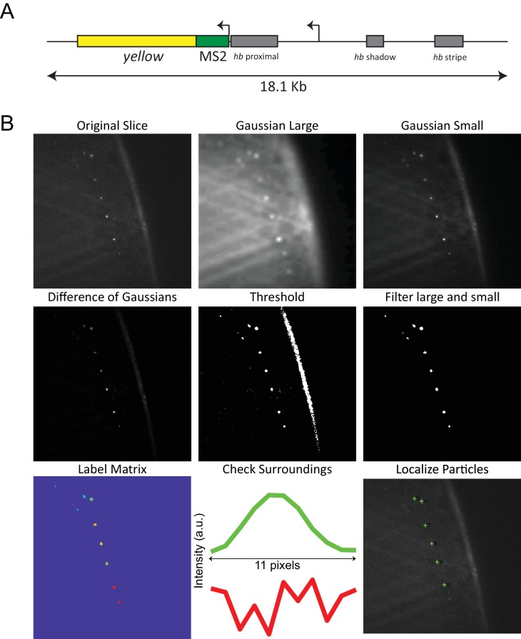
Figure 7u2014figure supplement 1.
MS2 system and data analysis.
( A ) BAC construct used in the experiments to visualize transcription of hb , from Bothma et al. (2015) . The coding region is replaced by the yellow gene and 24 MS2 stem loops are inserted downstrea...
Figure 7u2014videou00a01.
Four dimensional imaging of protein distribution in the context of transcription.
Related to Figure 7 .u00a0Example of four dimensional imaging of Zld spatial distribution in the context of an active transcription site imaged using the MS2-MCP system (red).
Figure 7u2014videou00a02.
Example of Bcd spatial distribution around an active hb locus.
Related to Figure 7 . eGFP-Bcd (green) and MCP-mcherry (red) dynamics from nuclear cycles 13u201314. Maximum intensity projection over 61 slices spaced 250 nm apart withu00a0~6 s between volumes.
Figure 7u2014videou00a03.
Example of Zld spatial distribution around an active hb locus.
Related to Figure 7 . mNeonGreen-Zld (green) and MCP-mcherry (red) dynamics from nuclear cycles 13u201314. Maximum intensity projection over 61 slices spaced 250 nm apart with 5.18 s between frames.
Figure 7u2014videou00a04.
Calculation of average Zld signal around active hb loci.
Related to Figure 7 .u00a0Top panel shows images of the MS2 signal, corresponding Zld signal in the same window (TS) and at a random control site in the same nucleus (RS). Middle panel shows a running...
Figure 7u2014videou00a05.
Calculation of average Bcd signal around active hb loci.
Related to Figure 7 .u00a0Top panel shows images of the MS2 signal, corresponding Bcd signal in the same window (TS) and at a random control site in the same nucleus (RS). Middle panel shows a running...
Author response image 1.
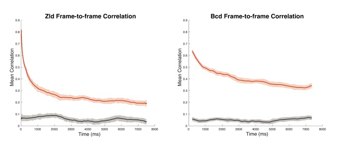
Frame-to-frame correlation of nuclear protein fluorescence generated from movies with a 15 ms frame rate for Zelda and 210 ms frame rate for Bcd.
Nuclei were manually segmented, fluorescent signal was normalized independently for each nucleus and each frame, and the pixel-wise correlation of nuclear signal between frames was calculated. Vectors...
Author responseu2014video 1.
Author response image 2.
Figure images are served from the NIH/NLM PubMed Central Open Access Subset or Europe PMC; copyright remains with the publishers and authors.
💬 Discussion
0 commentsNo comments yet. Be the first to start a discussion!
Leave a Comment