Abstract
Abstract How to deal with continuously flexing molecules is one of the biggest outstanding challenges in single-particle analysis of proteins from cryogenic-electron microscopy (cryo-EM) images. Here, we present DynaMight, a software tool that estimates a continuous space of conformations in a cryo-EM dataset by learning three-dimensional deformations of a Gaussian pseudo-atomic model of a consensus structure for every particle image. Inversion of the learned deformations is then used to obtain an improved reconstruction of the consensus structure. We illustrate the performance of DynaMight for several experimental cryo-EM datasets. We also show how error estimates on the deformations may be obtained by independently training two variational autoencoders on half sets of the cryo-EM data, and how regularization of the three-dimensional deformations through the use of atomic models may lead to important artifacts due to model bias. DynaMight is distributed as free, open-source software, as part of RELION-5.
🔬 Techniques
🧬 Organisms
🧪 Sample Preparation
🧪 Reagent Suppliers
💻 Software Details
💾 Data Repositories
🏛️ Research Organizations (ROR)
Affiliated research institutions:
📋 Methods
Initialization of the reference model
We model the 3D cryo-EM density map documentclass[12pt]{minimal} usepackage{amsmath} usepackage{wasysym} usepackage{amsfonts} usepackage{amssymb} usepackage{amsbsy} usepackage{mathrsfs} usepackage{upgreek} setlength{oddsidemargin}{-69pt} begin{document}$$f:{{mathbb{R}}}^{3}to {mathbb{R}}$$end{document} f : R 3 → R by a sum of N g Gaussian functions. The density f is defined by 8 documentclass[12pt]{minimal} usepackage{amsmath} usepackage{wasysym} usepackage{amsfonts} usepackage{amssymb} usepackage{amsbsy} usepackage{mathrsfs} usepackage{upgreek} setlength{oddsidemargin}{-69pt} begin{document}$$f({{{bf{x}}}})=sumlimits_{j=1}^{{N}_{mathrm{c}}}left(sumlimits_{i=1}^{{N}_{mathrm{g}}}{d}_{j,i}{a}_{j}exp left(frac{parallel {{{bf{x}}}}-{c}_{i}parallel }{{s}_{j}}right)right).$$end{document} f ( x ) = ∑ j = 1 N c ∑ i = 1 N g d j , i a j exp ∥ x − c i ∥ s j . Here N c is a fixed number defining how many distinct widths are used in the Gaussian model. For the i th Gaussian the vector d –, i satisfies documentclass[12pt]{minimal} usepackage{amsmath} usepackage{wasysym} usepackage{amsfonts} usepackage{amssymb} usepackage{amsbsy} usepackage{mathrsfs} usepackage{upgreek} setlength{oddsidemargin}{-69pt} begin{document}$$sumnolimits_{j=1}^{{N}_{mathrm{c}}}{d}_{j,i}=1$$end{document} ∑ j = 1 N c d j , i = 1 and d j , i ≥ 0 for all j ∈ {1, …, N c }. This weight vector continuously classifies the type of Gaussian that is selected for a certain position of the Gaussian model. Although we used N c = 1 in all our results, using more classes could be helpful for cases where the consensus map contains large variations in local resolution and the same width of all Gaussians does not give a reasonable representation of the map. The learnable parameters in this model are the widths documentclass[12pt]{minimal} usepackage{amsmath} usepackage{wasysym} usepackage{amsfonts} usepackage{amssymb} usepackage{amsbsy} usepackage{mathrsfs} usepackage{upgreek} setlength{oddsidemargin}{-69pt} begin{document}$$({s}_{1},ldots ,{s}_{{N}_{mathrm{c}}})$$end{document} ( s 1 , … , s N c ) , composition vectors d and amplitudes documentclass[12pt]{minimal} usepackage{amsmath} usepackage{wasysym} usepackage{amsfonts} usepackage{amssymb} usepackage{amsbsy} usepackage{mathrsfs} usepackage{upgreek} setlength{oddsidemargin}{-69pt} begin{document}$$({a}_{1},ldots ,{a}_{{N}_{mathrm{c}}})$$end{document} ( a 1 , … , a N c ) . These parameters are optimized globally, meaning that they are independent of the projection image, and stay the same over the whole dataset. Whereas a per-Gaussian amplitude parameter would be possible and would enable the representation of compositional heterogeneity, we decided to use the same amplitudes for all Gaussians. The reason for this is that otherwise movement could also be represented by Gaussian densities vanishing and reappearing at different places. We call the parameters ( a , s , d , c ) of the Gaussian model the reference parameters and we use a separate optimizer (ADAM) to update them. The total number of reference parameters is N g × 3 + N c × ( N g + 2). For our experiments, we used only one class of Gaussians, resulting in N g × 3 + 2 parameters. The consensus model serves as the starting point for the decoder that predicts how every Gaussian in the model moves to explain the corresponding experimental image. In the recommended way of running DynaMight, the initial reference map, that is, the reconstruction from the consensus refinement, is thresholded and randomly filled with N g Gaussians that are within the region of the map exceeding this threshold. The threshold should be chosen such that density in the flexible regions remains, but no noise is visible in the solvent region. The parameters a and s are initialized to reasonable numbers such that the norm of the Gaussian model equals the norm of the consensus reconstruction and the classification weights are initialized randomly. Once the reference parameters are initialized, we optimize the reference model using gradient descent (that is, without any networks), minimizing the mean squared error to the experimental images. Alternatively, Gaussians may be initialized from the positions of an atomic model that is rigid-body fitted into the consensus map. For our experiments with atomic models for the spliceosome dataset, we used the deposited atomic model (PDB 5nrl ). Instead of using one Gaussian per atom, we coarse-grained the atomic models. For every amino acid we used one main chain Gaussian that was located at the Bary center of the N, C and O atoms. Subsequent main chain Gaussians were connected by an edge in the graph used for regularization. The number of Gaussians used to represent the side chains varied for different amino acids. We placed one additional Gaussian at the Bary center of the α , β and γ position side-chain atoms of all amino acids, except for ‘PRO’, where we took the Bary center of atoms at the α , β , γ and δ positions, and for ‘SER’, ‘CYS’, ‘ALA’, ‘GLY’, ‘VAL’ and ‘THR’, where we placed a Gaussian at the β position. For larger amino acids, we placed additional side-chain Gaussians at the Bary center of the remaining side-chain atoms, except for ‘TYR’ and ‘TRP’, where we used two additional Gaussians. Subsequent Gaussians from the side chains were connected to each other and then to the corresponding main chain Gaussian with edges for the regularization functional. The amplitudes of the Gaussians were chosen to be proportional to the combined atomic number of all (nonhydrogen) atoms grouped together for the corresponding Gaussian. For nucleic acids we used four Gaussians: one at the phosphate position and one at the Bary center of the sugar form the main chain of the nucleic acid chain and two Gaussians at the bases. Again, the amplitudes were set to be proportional to the combined atomic number within each group. The VAE A VAE estimates displacements of the Gaussians from the reference model. An encoder learns an embedding to a low dimensional latent space that describes the conformational landscape of the dataset. The decoder estimates a deformation, given a point in that latent space and a position in the 3D reference. The input to the encoder is a flattened (real-space) experimental image y i and the output are two vectors documentclass[12pt]{minimal} usepackage{amsmath} usepackage{wasysym} usepackage{amsfonts} usepackage{amssymb} usepackage{amsbsy} usepackage{mathrsfs} usepackage{upgreek} setlength{oddsidemargin}{-69pt} begin{document}$$({mu }_{i},{sigma }_{i})in {{mathbb{R}}}^{{N}_{l}}times {{mathbb{R}}}^{{N}_{l}}$$end{document} ( μ i , σ i ) ∈ R N l × R N l , which describe the mean and standard deviation used to generate a sample, which serves as an input for the decoder. The encoder is a fully connected neural network with three linear layers and rectified linear unit activation functions. To optimize the weights of the encoder we used the ADAM optimizer with a learning rate of 0.001. We tried to use alternative encoder architectures using residual connections, more linear layers and convolutional neural networks, but without observing relevant improvements in performance. Even when substituting the input images with a different unique signal (we used a random vector per image), the deformations are not worse. We conclude that the encoder does not effectively use the information that is present in the images, suggesting that one could optimize the latent representation itself via an autodecoder 12 . The decoder is at the heart of our approach. Given a conformational representation it estimates a deformation for the corresponding particle image. It takes the latent representation z i and a spatial position, and outputs the displacement of that which is predicted at this spatial position. During training, the positions where the decoder is evaluated are the Gaussian positions in the reference model. Compared to ref. 10 we use a coordinate-based network that takes the input position as an input. To augment the 3D coordinates, we use positional encoding with ten encoding dimensions, which has shown to resolve higher resolution information in coordinate-based networks 31 . We use the sine and cosine function for lifting the 3D position to a higher dimensional space as described in ref. 32 . We observed that without the positional encoding of the input coordinate the deformations are too smooth and that localized motion is not captured well. The use of a coordinate-based network results in a network that approximates a deformation field that can be evaluated at any position in documentclass[12pt]{minimal} usepackage{amsmath} usepackage{wasysym} usepackage{amsfonts} usepackage{amssymb} usepackage{amsbsy} usepackage{mathrsfs} usepackage{upgreek} setlength{oddsidemargin}{-69pt} begin{document}$${{mathbb{R}}}^{3}$$end{document} R 3 . The decoder itself is a fully connected network δ with exponential linear unit (ELU) activation functions and an additive residual connection (Extended Data Fig. 1 ). We use eight linear layers to obtain for a given spatial position documentclass[12pt]{minimal} usepackage{amsmath} usepackage{wasysym} usepackage{amsfonts} usepackage{amssymb} usepackage{amsbsy} usepackage{mathrsfs} usepackage{upgreek} setlength{oddsidemargin}{-69pt} begin{document}$${{{bf{x}}}}in {{mathbb{R}}}^{3}$$end{document} x ∈ R 3 the deformed position: 9 documentclass[12pt]{minimal} usepackage{amsmath} usepackage{wasysym} usepackage{amsfonts} usepackage{amssymb} usepackage{amsbsy} usepackage{mathrsfs} usepackage{upgreek} setlength{oddsidemargin}{-69pt} begin{document}$$begin{array}{r}{{{mathcal{D}}}}({z}_{i},{{{bf{x}}}})={{{bf{x}}}}+delta ({z}_{i},{{{bf{x}}}}).end{array}$$end{document} D ( z i , x ) = x + δ ( z i , x ) . In the training phase, we evaluate the decoder for all the positions c 0 in the reference model. We then model the forward operator of cryo-EM by projecting the center points of the deformed Gaussian reference model using the orientation of the particle, resulting in 2D coordinates ξ i . These coordinates are then placed into an (oversampled) 2D grid using bilinear interpolation. Then we compute the 2D Fourier transform, approximating the Fourier transform of the sum of deltas. Subsequently, we multiply the resulting Fourier-space image with the Gaussian basis function G s and the CTF documentclass[12pt]{minimal} usepackage{amsmath} usepackage{wasysym} usepackage{amsfonts} usepackage{amssymb} usepackage{amsbsy} usepackage{mathrsfs} usepackage{upgreek} setlength{oddsidemargin}{-69pt} begin{document}$${{{{mathcal{C}}}}}_{i}$$end{document} C i resulting in the projection image g i of the deformed Gaussian model 10 documentclass[12pt]{minimal} usepackage{amsmath} usepackage{wasysym} usepackage{amsfonts} usepackage{amssymb} usepackage{amsbsy} usepackage{mathrsfs} usepackage{upgreek} setlength{oddsidemargin}{-69pt} begin{document}$${g}_{i}approx {{{mathcal{F}}}}left(sumlimits_{j=1}^{{N}_{mathrm{g}}}a{delta }_{{xi }_{i}^{j}}right)cdot {{{{mathcal{C}}}}}_{i}cdot {G}_{mathrm{s}}.$$end{document} g i ≈ F ∑ j = 1 N g a δ ξ i j ⋅ C i ⋅ G s . If more than one type of Gaussian exists, the same operation is repeated for all types and weighted by the class assignment vector d . The resulting reference projection image g i is then compared to the experimental image, using a mean squared error as the loss function (also below).
Show full methods section
Initialization of the reference model
We model the 3D cryo-EM density map documentclass[12pt]{minimal} usepackage{amsmath} usepackage{wasysym} usepackage{amsfonts} usepackage{amssymb} usepackage{amsbsy} usepackage{mathrsfs} usepackage{upgreek} setlength{oddsidemargin}{-69pt} begin{document}$$f:{{mathbb{R}}}^{3}to {mathbb{R}}$$end{document} f : R 3 → R by a sum of N g Gaussian functions. The density f is defined by 8 documentclass[12pt]{minimal} usepackage{amsmath} usepackage{wasysym} usepackage{amsfonts} usepackage{amssymb} usepackage{amsbsy} usepackage{mathrsfs} usepackage{upgreek} setlength{oddsidemargin}{-69pt} begin{document}$$f({{{bf{x}}}})=sumlimits_{j=1}^{{N}_{mathrm{c}}}left(sumlimits_{i=1}^{{N}_{mathrm{g}}}{d}_{j,i}{a}_{j}exp left(frac{parallel {{{bf{x}}}}-{c}_{i}parallel }{{s}_{j}}right)right).$$end{document} f ( x ) = ∑ j = 1 N c ∑ i = 1 N g d j , i a j exp ∥ x − c i ∥ s j . Here N c is a fixed number defining how many distinct widths are used in the Gaussian model. For the i th Gaussian the vector d –, i satisfies documentclass[12pt]{minimal} usepackage{amsmath} usepackage{wasysym} usepackage{amsfonts} usepackage{amssymb} usepackage{amsbsy} usepackage{mathrsfs} usepackage{upgreek} setlength{oddsidemargin}{-69pt} begin{document}$$sumnolimits_{j=1}^{{N}_{mathrm{c}}}{d}_{j,i}=1$$end{document} ∑ j = 1 N c d j , i = 1 and d j , i ≥ 0 for all j ∈ {1, …, N c }. This weight vector continuously classifies the type of Gaussian that is selected for a certain position of the Gaussian model. Although we used N c = 1 in all our results, using more classes could be helpful for cases where the consensus map contains large variations in local resolution and the same width of all Gaussians does not give a reasonable representation of the map. The learnable parameters in this model are the widths documentclass[12pt]{minimal} usepackage{amsmath} usepackage{wasysym} usepackage{amsfonts} usepackage{amssymb} usepackage{amsbsy} usepackage{mathrsfs} usepackage{upgreek} setlength{oddsidemargin}{-69pt} begin{document}$$({s}_{1},ldots ,{s}_{{N}_{mathrm{c}}})$$end{document} ( s 1 , … , s N c ) , composition vectors d and amplitudes documentclass[12pt]{minimal} usepackage{amsmath} usepackage{wasysym} usepackage{amsfonts} usepackage{amssymb} usepackage{amsbsy} usepackage{mathrsfs} usepackage{upgreek} setlength{oddsidemargin}{-69pt} begin{document}$$({a}_{1},ldots ,{a}_{{N}_{mathrm{c}}})$$end{document} ( a 1 , … , a N c ) . These parameters are optimized globally, meaning that they are independent of the projection image, and stay the same over the whole dataset. Whereas a per-Gaussian amplitude parameter would be possible and would enable the representation of compositional heterogeneity, we decided to use the same amplitudes for all Gaussians. The reason for this is that otherwise movement could also be represented by Gaussian densities vanishing and reappearing at different places. We call the parameters ( a , s , d , c ) of the Gaussian model the reference parameters and we use a separate optimizer (ADAM) to update them. The total number of reference parameters is N g × 3 + N c × ( N g + 2). For our experiments, we used only one class of Gaussians, resulting in N g × 3 + 2 parameters. The consensus model serves as the starting point for the decoder that predicts how every Gaussian in the model moves to explain the corresponding experimental image. In the recommended way of running DynaMight, the initial reference map, that is, the reconstruction from the consensus refinement, is thresholded and randomly filled with N g Gaussians that are within the region of the map exceeding this threshold. The threshold should be chosen such that density in the flexible regions remains, but no noise is visible in the solvent region. The parameters a and s are initialized to reasonable numbers such that the norm of the Gaussian model equals the norm of the consensus reconstruction and the classification weights are initialized randomly. Once the reference parameters are initialized, we optimize the reference model using gradient descent (that is, without any networks), minimizing the mean squared error to the experimental images. Alternatively, Gaussians may be initialized from the positions of an atomic model that is rigid-body fitted into the consensus map. For our experiments with atomic models for the spliceosome dataset, we used the deposited atomic model (PDB 5nrl ). Instead of using one Gaussian per atom, we coarse-grained the atomic models. For every amino acid we used one main chain Gaussian that was located at the Bary center of the N, C and O atoms. Subsequent main chain Gaussians were connected by an edge in the graph used for regularization. The number of Gaussians used to represent the side chains varied for different amino acids. We placed one additional Gaussian at the Bary center of the α , β and γ position side-chain atoms of all amino acids, except for ‘PRO’, where we took the Bary center of atoms at the α , β , γ and δ positions, and for ‘SER’, ‘CYS’, ‘ALA’, ‘GLY’, ‘VAL’ and ‘THR’, where we placed a Gaussian at the β position. For larger amino acids, we placed additional side-chain Gaussians at the Bary center of the remaining side-chain atoms, except for ‘TYR’ and ‘TRP’, where we used two additional Gaussians. Subsequent Gaussians from the side chains were connected to each other and then to the corresponding main chain Gaussian with edges for the regularization functional. The amplitudes of the Gaussians were chosen to be proportional to the combined atomic number of all (nonhydrogen) atoms grouped together for the corresponding Gaussian. For nucleic acids we used four Gaussians: one at the phosphate position and one at the Bary center of the sugar form the main chain of the nucleic acid chain and two Gaussians at the bases. Again, the amplitudes were set to be proportional to the combined atomic number within each group. The VAE A VAE estimates displacements of the Gaussians from the reference model. An encoder learns an embedding to a low dimensional latent space that describes the conformational landscape of the dataset. The decoder estimates a deformation, given a point in that latent space and a position in the 3D reference. The input to the encoder is a flattened (real-space) experimental image y i and the output are two vectors documentclass[12pt]{minimal} usepackage{amsmath} usepackage{wasysym} usepackage{amsfonts} usepackage{amssymb} usepackage{amsbsy} usepackage{mathrsfs} usepackage{upgreek} setlength{oddsidemargin}{-69pt} begin{document}$$({mu }_{i},{sigma }_{i})in {{mathbb{R}}}^{{N}_{l}}times {{mathbb{R}}}^{{N}_{l}}$$end{document} ( μ i , σ i ) ∈ R N l × R N l , which describe the mean and standard deviation used to generate a sample, which serves as an input for the decoder. The encoder is a fully connected neural network with three linear layers and rectified linear unit activation functions. To optimize the weights of the encoder we used the ADAM optimizer with a learning rate of 0.001. We tried to use alternative encoder architectures using residual connections, more linear layers and convolutional neural networks, but without observing relevant improvements in performance. Even when substituting the input images with a different unique signal (we used a random vector per image), the deformations are not worse. We conclude that the encoder does not effectively use the information that is present in the images, suggesting that one could optimize the latent representation itself via an autodecoder 12 . The decoder is at the heart of our approach. Given a conformational representation it estimates a deformation for the corresponding particle image. It takes the latent representation z i and a spatial position, and outputs the displacement of that which is predicted at this spatial position. During training, the positions where the decoder is evaluated are the Gaussian positions in the reference model. Compared to ref. 10 we use a coordinate-based network that takes the input position as an input. To augment the 3D coordinates, we use positional encoding with ten encoding dimensions, which has shown to resolve higher resolution information in coordinate-based networks 31 . We use the sine and cosine function for lifting the 3D position to a higher dimensional space as described in ref. 32 . We observed that without the positional encoding of the input coordinate the deformations are too smooth and that localized motion is not captured well. The use of a coordinate-based network results in a network that approximates a deformation field that can be evaluated at any position in documentclass[12pt]{minimal} usepackage{amsmath} usepackage{wasysym} usepackage{amsfonts} usepackage{amssymb} usepackage{amsbsy} usepackage{mathrsfs} usepackage{upgreek} setlength{oddsidemargin}{-69pt} begin{document}$${{mathbb{R}}}^{3}$$end{document} R 3 . The decoder itself is a fully connected network δ with exponential linear unit (ELU) activation functions and an additive residual connection (Extended Data Fig. 1 ). We use eight linear layers to obtain for a given spatial position documentclass[12pt]{minimal} usepackage{amsmath} usepackage{wasysym} usepackage{amsfonts} usepackage{amssymb} usepackage{amsbsy} usepackage{mathrsfs} usepackage{upgreek} setlength{oddsidemargin}{-69pt} begin{document}$${{{bf{x}}}}in {{mathbb{R}}}^{3}$$end{document} x ∈ R 3 the deformed position: 9 documentclass[12pt]{minimal} usepackage{amsmath} usepackage{wasysym} usepackage{amsfonts} usepackage{amssymb} usepackage{amsbsy} usepackage{mathrsfs} usepackage{upgreek} setlength{oddsidemargin}{-69pt} begin{document}$$begin{array}{r}{{{mathcal{D}}}}({z}_{i},{{{bf{x}}}})={{{bf{x}}}}+delta ({z}_{i},{{{bf{x}}}}).end{array}$$end{document} D ( z i , x ) = x + δ ( z i , x ) . In the training phase, we evaluate the decoder for all the positions c 0 in the reference model. We then model the forward operator of cryo-EM by projecting the center points of the deformed Gaussian reference model using the orientation of the particle, resulting in 2D coordinates ξ i . These coordinates are then placed into an (oversampled) 2D grid using bilinear interpolation. Then we compute the 2D Fourier transform, approximating the Fourier transform of the sum of deltas. Subsequently, we multiply the resulting Fourier-space image with the Gaussian basis function G s and the CTF documentclass[12pt]{minimal} usepackage{amsmath} usepackage{wasysym} usepackage{amsfonts} usepackage{amssymb} usepackage{amsbsy} usepackage{mathrsfs} usepackage{upgreek} setlength{oddsidemargin}{-69pt} begin{document}$${{{{mathcal{C}}}}}_{i}$$end{document} C i resulting in the projection image g i of the deformed Gaussian model 10 documentclass[12pt]{minimal} usepackage{amsmath} usepackage{wasysym} usepackage{amsfonts} usepackage{amssymb} usepackage{amsbsy} usepackage{mathrsfs} usepackage{upgreek} setlength{oddsidemargin}{-69pt} begin{document}$${g}_{i}approx {{{mathcal{F}}}}left(sumlimits_{j=1}^{{N}_{mathrm{g}}}a{delta }_{{xi }_{i}^{j}}right)cdot {{{{mathcal{C}}}}}_{i}cdot {G}_{mathrm{s}}.$$end{document} g i ≈ F ∑ j = 1 N g a δ ξ i j ⋅ C i ⋅ G s . If more than one type of Gaussian exists, the same operation is repeated for all types and weighted by the class assignment vector d . The resulting reference projection image g i is then compared to the experimental image, using a mean squared error as the loss function (also below).
Training
After initialization of the Gaussians in the consensus reconstruction, during the first epochs (that is, sweeps over the two half sets for both models) of training we only optimize the Gaussian parameters, that is their widths, amplitudes and positions. After this initial phase, we also start optimizing the network parameters of the two independent VAEs, which are initially assigned random values. Both phases of training use the ADAM optimizer at a learning rate 0.0001. To get physically meaningful deformations, the reference model itself should lie within the distribution of all the conformations estimated by the decoder, rather than being a nonexisting average of conformations (as the reconstruction from the consensus refinement is). To achieve this, we apply two heuristic strategies that gradually improve the reference model. First, after every 30 epochs, we fix the encoder and decoder for five epochs and only adjust the Gaussian parameters. Second, at every tenth epoch where the decoder is not fixed, we replace the positions of the Gaussians of the reference model by the predicted Gaussian positions with the smallest displacement from the current reference model. The latter ensures that the reference model is in the distribution of deformed models. Without this replacement strategy, we observed that the reference model can move out of distribution, sometimes even to a point where the structure is completely distorted. As long as the deformations satisfy the regularization constraints, this should not change the value of the loss function, but we observed that this can lead to unphysical displacements of the Gaussians and suboptimal reconstructions. To also ensure that the reference models of the two independent half sets are in the same conformation, we generate a binary mask around the Gaussians positions of one half set and substitute the Gaussian positions of the other half set with the average over 100 predictions where the number of Gaussians inside this mask is the highest. The binary mask covers all voxels that have a Gaussian within a distance of 6 Å from the voxel center. Fourier shell correlations of the Gaussian model to the consensus and the final Gaussian model to the final reconstruction are displayed in Supplementary Fig. 1 . Training is stopped when the updates of the consensus model do not yield improvements in the data loss mean squared error (MSE; below) anymore. More specifically, we stop training if the MSE loss increased for the k th time. In our experiments we used the default value of k = 40. Loss functions and regularization Denoting by g i the reference projection image generated by the current VAE, the main loss function is the data loss, which for a batch documentclass[12pt]{minimal} usepackage{amsmath} usepackage{wasysym} usepackage{amsfonts} usepackage{amssymb} usepackage{amsbsy} usepackage{mathrsfs} usepackage{upgreek} setlength{oddsidemargin}{-69pt} begin{document}$${{{mathcal{B}}}}:={({g}_{i},{y}_{i})}_{iin {{{bf{B}}}}}$$end{document} B : = ( g i , y i ) i ∈ B is computed in Fourier space as 11 documentclass[12pt]{minimal} usepackage{amsmath} usepackage{wasysym} usepackage{amsfonts} usepackage{amssymb} usepackage{amsbsy} usepackage{mathrsfs} usepackage{upgreek} setlength{oddsidemargin}{-69pt} begin{document}$$begin{array}{r}{{{mathcal{F}}}}({{{mathcal{B}}}}):=frac{1}{| {{{mathcal{B}}}}| }sumlimits_{iin {{{mathcal{B}}}}}parallel {g}_{i}-{y}_{i}{parallel }_{{{varSigma }}}^{2},end{array}$$end{document} F ( B ) : = 1 ∣ B ∣ ∑ i ∈ B ∥ g i − y i ∥ Σ 2 , where the resolution-dependent noise weights Σ are estimated by the radially averaged power of the error on a subset of particle images. Auxiliary losses are used to regularize the deformations of the Gaussian model. In the recommended way of running DynaMight, a graph is constructed by connecting Gaussians that are within a certain distance with edges. The set of edges is defined by 12 documentclass[12pt]{minimal} usepackage{amsmath} usepackage{wasysym} usepackage{amsfonts} usepackage{amssymb} usepackage{amsbsy} usepackage{mathrsfs} usepackage{upgreek} setlength{oddsidemargin}{-69pt} begin{document}$$begin{array}{r}{E}_{ij}=left{begin{array}{ll}1quad quad ¶llel {c}_{i}-{c}_{j}parallel < 1.5,{c}_{{{{rm{mean}}}}},\ 0quad &{{{rm{else.}}}}end{array}right.end{array}$$end{document} E i j = 1 ∥ c i − c j ∥ < 1.5 c mean , 0 else. Here c mean is the mean distance in the graph F i j , which is created by connecting every point to its two nearest neighbors. These graphs are recalculated from the reference model after every epoch. For the deformation of the k th image Γ k the following regularization functional then preserves distances after displacement, enforcing local isometry: 13 documentclass[12pt]{minimal} usepackage{amsmath} usepackage{wasysym} usepackage{amsfonts} usepackage{amssymb} usepackage{amsbsy} usepackage{mathrsfs} usepackage{upgreek} setlength{oddsidemargin}{-69pt} begin{document}$${{{{mathcal{R}}}}}_{d}({{{varGamma }}}_{k})=sumlimits_{{(i,,j):{E}_{ij}=1}}{leftvert parallel {c}_{i}-{c}_{j}parallel -parallel {{{varGamma }}}_{k}({c}_{i})-{{{varGamma }}}_{k}({c}_{j})parallel rightvert }^{2},$$end{document} R d ( Γ k ) = ∑ { ( i , j ) : E i j = 1 } ∥ c i − c j ∥ − ∥ Γ k ( c i ) − Γ k ( c j ) ∥ 2 , Additionally, we use a repulsion loss penalizing Gaussians that are too close to each other 14 documentclass[12pt]{minimal} usepackage{amsmath} usepackage{wasysym} usepackage{amsfonts} usepackage{amssymb} usepackage{amsbsy} usepackage{mathrsfs} usepackage{upgreek} setlength{oddsidemargin}{-69pt} begin{document}$${{{{mathcal{R}}}}}_{r}({{{varGamma }}}_{k})=sumlimits_{{(i,,j):{E}_{ij}=1}}{chi }_{parallel {{{varGamma }}}_{k}({c}_{i})-{{{varGamma }}}_{k}({c}_{j})parallel < tau }{(parallel {{{varGamma }}}_{k}({c}_{i})-{{{varGamma }}}_{k}({c}_{j})parallel -tau )}^{2},$$end{document} R r ( Γ k ) = ∑ { ( i , j ) : E i j = 1 } χ ∥ Γ k ( c i ) − Γ k ( c j ) ∥ < τ ( ∥ Γ k ( c i ) − Γ k ( c j ) ∥ − τ ) 2 , where documentclass[12pt]{minimal} usepackage{amsmath} usepackage{wasysym} usepackage{amsfonts} usepackage{amssymb} usepackage{amsbsy} usepackage{mathrsfs} usepackage{upgreek} setlength{oddsidemargin}{-69pt} begin{document}$${chi }_{parallel {{varGamma }}({c}_{i})-{{varGamma }}({c}_{j})parallel < tau }$$end{document} χ ∥ Γ ( c i ) − Γ ( c j ) ∥ < τ = 1 if the distance between neighboring Gaussians is less than τ . We set τ to c mean for all our results. The total loss function is then given by documentclass[12pt]{minimal} usepackage{amsmath} usepackage{wasysym} usepackage{amsfonts} usepackage{amssymb} usepackage{amsbsy} usepackage{mathrsfs} usepackage{upgreek} setlength{oddsidemargin}{-69pt} begin{document}$${{{mathcal{L}}}}({{{mathcal{B}}}})={{{mathcal{F}}}}({{{mathcal{B}}}})+lambda frac{1}{| {{{mathcal{B}}}}| }sumlimits_{iin {{{mathcal{B}}}}}left[{{{{mathcal{R}}}}}_{d}({{{varGamma }}}_{i})+{{{{mathcal{R}}}}}_{r}({{{varGamma }}}_{k})right]=:{{{mathcal{F}}}}({{{mathcal{B}}}})+lambda {{{mathcal{R}}}}({{{mathcal{B}}}}).$$end{document} L ( B ) = F ( B ) + λ 1 ∣ B ∣ ∑ i ∈ B R d ( Γ i ) + R r ( Γ k ) = : F ( B ) + λ R ( B ) . The parameter λ is a dynamic regularization parameter that is recalculated after every epoch. We do that by calculating the norm of the gradients of both loss terms documentclass[12pt]{minimal} usepackage{amsmath} usepackage{wasysym} usepackage{amsfonts} usepackage{amssymb} usepackage{amsbsy} usepackage{mathrsfs} usepackage{upgreek} setlength{oddsidemargin}{-69pt} begin{document}$${{{mathcal{L}}}}$$end{document} L and documentclass[12pt]{minimal} usepackage{amsmath} usepackage{wasysym} usepackage{amsfonts} usepackage{amssymb} usepackage{amsbsy} usepackage{mathrsfs} usepackage{upgreek} setlength{oddsidemargin}{-69pt} begin{document}$${{{mathcal{R}}}}$$end{document} R and define λ such that the ratio of these norms equal a user-defined number. When set to 1 the norm of the gradient of both terms is equal. For all our results we set this value to 0.9, which results in slightly more influence of the data term documentclass[12pt]{minimal} usepackage{amsmath} usepackage{wasysym} usepackage{amsfonts} usepackage{amssymb} usepackage{amsbsy} usepackage{mathrsfs} usepackage{upgreek} setlength{oddsidemargin}{-69pt} begin{document}$${{{mathcal{L}}}}$$end{document} L . For the results, where we used the coarse-grained atomic model as a reference, we used the same data loss function documentclass[12pt]{minimal} usepackage{amsmath} usepackage{wasysym} usepackage{amsfonts} usepackage{amssymb} usepackage{amsbsy} usepackage{mathrsfs} usepackage{upgreek} setlength{oddsidemargin}{-69pt} begin{document}$${{{mathcal{F}}}}$$end{document} F (equation ( 12 )), but in contrast to the above described heuristic method to construct the edges between the Gaussian, the graph E is obtained from the coarse graining of the atomic model. The regularization that preserves distances is applied in the same way (equation ( 13 )) with the fixed graph from the coarse graining. The second regularization functional (equation ( 14 )) is not used in this case, since the distances in the reference model are fixed.
Improved reconstruction
To calculate an improved reconstruction from the estimated deformations, we use a network documentclass[12pt]{minimal} usepackage{amsmath} usepackage{wasysym} usepackage{amsfonts} usepackage{amssymb} usepackage{amsbsy} usepackage{mathrsfs} usepackage{upgreek} setlength{oddsidemargin}{-69pt} begin{document}$${{{{mathcal{D}}}}}^{-1}$$end{document} D − 1 with the same architecture as the decoder to estimate a deformation field that maps back a deformed position to its original location. Again this network is coordinate-based and can be evaluated on an arbitrary position documentclass[12pt]{minimal} usepackage{amsmath} usepackage{wasysym} usepackage{amsfonts} usepackage{amssymb} usepackage{amsbsy} usepackage{mathrsfs} usepackage{upgreek} setlength{oddsidemargin}{-69pt} begin{document}$${{{bf{x}}}}in {{mathbb{R}}}^{3}$$end{document} x ∈ R 3 . Given the latent representation of each particle we train the neural network documentclass[12pt]{minimal} usepackage{amsmath} usepackage{wasysym} usepackage{amsfonts} usepackage{amssymb} usepackage{amsbsy} usepackage{mathrsfs} usepackage{upgreek} setlength{oddsidemargin}{-69pt} begin{document}$${{{{mathcal{D}}}}}^{-1}$$end{document} D − 1 to map back the positions predicted by the trained VAE to the positions of the reference model. Since the model should estimate the inverse deformation of the decoder documentclass[12pt]{minimal} usepackage{amsmath} usepackage{wasysym} usepackage{amsfonts} usepackage{amssymb} usepackage{amsbsy} usepackage{mathrsfs} usepackage{upgreek} setlength{oddsidemargin}{-69pt} begin{document}$${{{mathcal{D}}}}$$end{document} D , it should satisfy documentclass[12pt]{minimal} usepackage{amsmath} usepackage{wasysym} usepackage{amsfonts} usepackage{amssymb} usepackage{amsbsy} usepackage{mathrsfs} usepackage{upgreek} setlength{oddsidemargin}{-69pt} begin{document}$$begin{array}{r}{{{{mathcal{D}}}}}^{-1}left(,{mu }_{i},{{{mathcal{D}}}}left({z}_{i},{c}_{j}^{0}right)right)={c}_{j}^{0}.end{array}$$end{document} D − 1 μ i , D z i , c j 0 = c j 0 . For each image g i the neural network takes as input the latent representation μ i from the previously trained encoder documentclass[12pt]{minimal} usepackage{amsmath} usepackage{wasysym} usepackage{amsfonts} usepackage{amssymb} usepackage{amsbsy} usepackage{mathrsfs} usepackage{upgreek} setlength{oddsidemargin}{-69pt} begin{document}$${{{mathcal{E}}}}$$end{document} E and a positional encoding of the deformed Gaussian positions documentclass[12pt]{minimal} usepackage{amsmath} usepackage{wasysym} usepackage{amsfonts} usepackage{amssymb} usepackage{amsbsy} usepackage{mathrsfs} usepackage{upgreek} setlength{oddsidemargin}{-69pt} begin{document}$${{{mathcal{D}}}}({z}_{i},{{{{bf{c}}}}}^{{{{{0}}}}})$$end{document} D ( z i , c 0 ) . The concatenated positional encoding and latent representation are then mapped by an multilayer perceptron with six layers and a single additive residual connection to the original coordinates of the consensus model c 0 . The loss function is the L 2 distance between the positions documentclass[12pt]{minimal} usepackage{amsmath} usepackage{wasysym} usepackage{amsfonts} usepackage{amssymb} usepackage{amsbsy} usepackage{mathrsfs} usepackage{upgreek} setlength{oddsidemargin}{-69pt} begin{document}$$begin{array}{r}frac{1}{{N}_{d}{N}_{mathrm{g}}}sumlimits_{i=1}^{{N}_{d}}sumlimits_{j=1}^{{N}_{mathrm{g}}}leftVert{{{{mathcal{D}}}}}^{-1}left(,{mu }_{i},{{{mathcal{D}}}}left({z}_{i},{c}_{j}^{0}right)right)-{c}_{j}^{0}rightVert^{2}end{array}$$end{document} 1 N d N g ∑ i = 1 N d ∑ j = 1 N g D − 1 μ i , D z i , c j 0 − c j 0 2 We optimized the weights of the inverse deformation network for 200 epochs with the ADAM optimizer for all our results. Once the network has been trained, the backprojection algorithm evaluates it for the latent representation of every particle on a 3D grid and applies the deformation to the CTF-multiplied, backprojected image. For computational speed, we evaluated the inverse deformation on a two times coarser grid, and then up-sampled the deformation fields to the original box size again using bilinear interpolation. The resulting volumes are then summed up and divided by the backprojected squared CTFs as illustrated in Fig. 1 . Reporting summary Further information on research design is available in the Nature Portfolio Reporting Summary linked to this article.
Online content Any methods, additional references, Nature Portfolio reporting summaries, source data, extended data, supplementary information, acknowledgements, peer review information; details of author contributions and competing interests; and statements of data and code availability are available at 10.1038/s41592-024-02377-5.
Supplementary information Supplementary Information Supplementary Table 1, Fig. 1 and Legends for Videos 1–6. Reporting Summary Peer Review File Supplementary Video 1 The video shows the DynaMight reconstructions with deformations obtained with the prior used from the correct atomic model (right) and the atomic model with an incorrect SF3a domain (left). The reconstructed density with the wrong prior clearly resembles the incorrect model. Supplementary Video 2 The video shows the DynaMight reconstructions with deformations obtained with the prior used from the correct atomic model (right) and the atomic model with an incorrect SF3b domain (left). For this better resolved region, the resemblance to the incorrect model is weaker than in Supplementary Video 1. Supplementary Video 3 The video shows a trajectory through latent space of half 1 for a subset of the EMPIAR-10180 dataset. The trajectory was chosen such that it covers disparate regions in latent space. Supplementary Video 4 The video shows a trajectory through latent space of half 1 for the 86,624 selected particles of the EMPIAR-10073 dataset. The trajectory was chosen such that it disparate regions in latent space. Supplementary Video 5 The video shows a trajectory through latent space of half 1 for the EMPIAR-11910 dataset. The trajectory was chosen such that it covers disparate regions in latent space. Supplementary Video 6 The video shows a trajectory through latent space of half 1 for the EMPIAR-11890 dataset. The trajectory was chosen such that it covers disparate regions in latent space.
Supplementary information The online version contains supplementary material available at 10.1038/s41592-024-02377-5.
📊 Figures
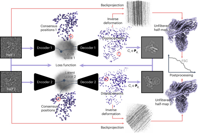
Fig. 1
Schematic illustration of DynaMight.
Two separate encoders take experimental images from each half set as input, and output a latent vector describing their conformational state. The decoders take the latent vectors together with the coo...
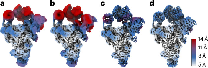
Fig. 2
DynaMight reconstructions of the spliceosome subset.
a , Standard RELION consensus refinement. b , DynaMight without regularization. c , DynaMight with smoothness regularization on the Gaussians. d , DynaMight with regularization from an atomic model. A...
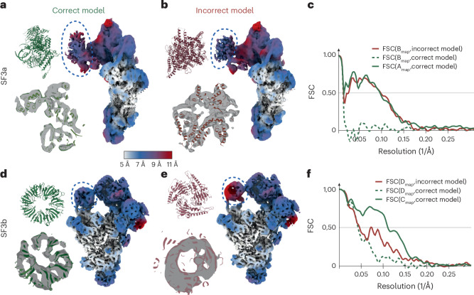
Fig. 3
Using incorrect atomic models in DynaMight.
a , Reconstruction after deformed backprojection using the correct atomic model for the SF3a region, colored by local resolution (right). The correct atomic model for the SF3a region is shown in green...
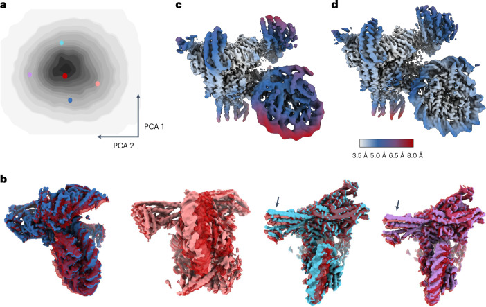
Fig. 4
DynaMight results for the CCANu2013CENP-A complex.
a , Principal components analysis (PCA) of the conformational latent space, with colored dots indicating the positions of the five maps in b . (Only the latent space for one of the two half sets is sh...
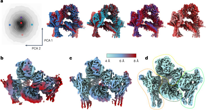
Fig. 5
DynaMight results for the complete kinetochore complex.
a , PCA of the conformational space (on the left) with highlighted positions of five conformation states, the maps of which are shown in the same colors on the right. (Only the latent space for one of...
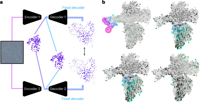
Fig. 6
Error estimation for the deformations.
a , Particles of a validation subset (here 10% of the particles) are fed into both encoders. The encoders are updated, whereas these images are not used for training the decoder. At evaluation time, b...
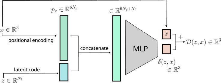
Extended Data Fig. 1
Diagram of the decoder architecture.
The queried position is lifted to a higher dimensional space via a fixed positional encoding function, where the lifting dimension is defined by Np. The Nl dimensional latent code is concatenated with...
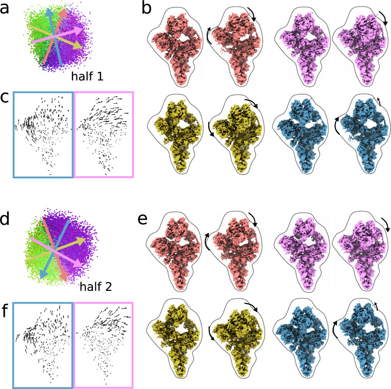
Extended Data Fig. 2
nalysis of motions for the pre-catalytic spliceosome.
a , d ) Latent spaces of both half sets (half 1 and half 2) for the pre-catalytic spliceosome dataset EMPIAR-( 10180 ) are coloured by the mean movement direction. Four different deformations are visu...
Extended Data Fig. 3
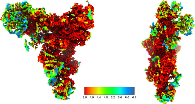
DynaMight reconstruction for the spliceosomal tri- snRNP complex.
The DynaMight reconstruction from 86,624 selected particles of data set EMPIAR- 10073 is coloured by local resolution, as estimated using cryoSPARC. The map is displayed in two orthogonal orientations...
Extended Data Fig. 4
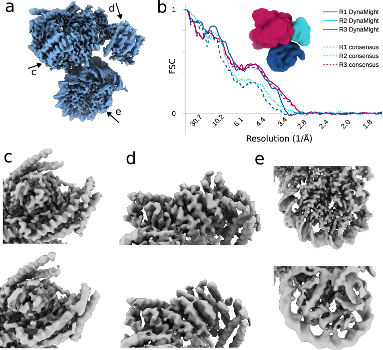
DynaMight reconstruction for the CCAN:CENP-A complex.
a ) Local resolution filtered map of the DynaMight reconstruction. b ) Fourier shell correlation (FSC) between atomic models fitted into 3 regions of the maps (R1-R3) and the DynaMight and consensus r...
Extended Data Fig. 5
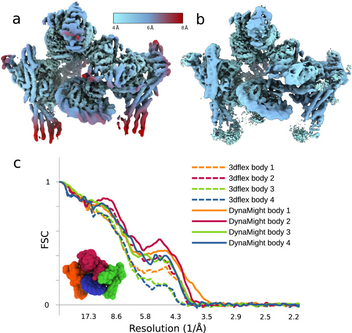
Comparison between DynaMight and 3DFlex for the kinetochore complex.
a , b ) Reconstructions from DynaMight ( a ) and 3DFlex ( b ), coloured according to local resolution (as estimated in RELION) with the same colour scheme, ranging from cyan (4 u2218 A) to red (8 u221...
Figure images are served from the NIH/NLM PubMed Central Open Access Subset or Europe PMC; copyright remains with the publishers and authors.
💬 Discussion
0 commentsNo comments yet. Be the first to start a discussion!
Leave a Comment