Abstract
Abstract The cell cycle is canonically described as a series of four consecutive phases: G1, S, G2, and M. In single cells, the duration of each phase varies, but the quantitative laws that govern phase durations are not well understood. Using time‐lapse microscopy, we found that each phase duration follows an Erlang distribution and is statistically independent from other phases. We challenged this observation by perturbing phase durations through oncogene activation, inhibition of DNA synthesis, reduced temperature, and DNA damage. Despite large changes in durations in cell populations, phase durations remained uncoupled in individual cells. These results suggested that the independence of phase durations may arise from a large number of molecular factors that each exerts a minor influence on the rate of cell cycle progression. We tested this model by experimentally forcing phase coupling through inhibition of cyclin‐dependent kinase 2 (CDK2) or overexpression of cyclin D. Our work provides an explanation for the historical observation that phase durations are both inherited and independent and suggests how cell cycle progression may be altered in disease states.
🔬 Techniques
🔭 Microscopes
🧬 Organisms
✨ Fluorophores
🧪 Sample Preparation
🔬 Cell Lines
🏭 Microscope Brands
🧪 Reagent Suppliers
📷 Detectors
🔎 Objectives
💻 Software Details
💾 Data Repositories
🏛️ Research Organizations (ROR)
Affiliated research institutions:
📋 Methods
Cell culture hTERT retinal pigment epithelial cells
(RPE) were obtained from the ATCC (ATCC® CRL‐4000™) and cultured in DMEM supplemented with 10% fetal calf serum (FBS) and penicillin/streptomycin. U2OS cells were obtained from the laboratory of Dr. Yue Xiong and cultured in DMEM supplemented with 10% fetal bovine serum (FBS) and penicillin/streptomycin (Gibco). WA09 (H9) hES cell line was purchased from WiCell (Wisconsin) and maintained in mTeSR1 (85850, StemCell Technologies) on growth factor reduced Matrigel (354230, BD). Cells were authenticated by STR profiling (ATCC, Manassas, VA) and confirmed to be free of mycoplasma. Cells were passaged using trypsin (25300054, Gibco) for RPE and U2OS or ReLeSR™ (05872, StemCell Technologies) for H9 as needed. When required, the medium was supplemented with selective antibiotics (2 μg/ml puromycin for RPE and U2OS; 0.5 μg/ml puromycin for H9; A1113803, Gibco). Chemical and genetic perturbation of the cell cycle phases For NCS treatment, medium was replaced with fresh medium supplemented with neocarzinostatin (N9162, Sigma‐Aldrich) during experiments. For myc overexpression, RPE cells were infected with fresh retrovirus containing MSCV‐Myc‐ER‐IRES‐GFP and 1 μl polybrene. Cells were subsequently passaged 48 of post‐infection and seeded onto a glass‐bottom plate for imaging. 16 h prior to imaging, tamoxifen was added at a final concentration of 50 nM. For aphidicolin treatment, medium was replaced with fresh medium supplemented with aphidicolin (A0781, Sigma‐Aldrich) for 8 h during experiments, washed off once with PBS, and then replenished with imaging media described below. For CDK2 inhibition, cells were treated with 2 μM CVT‐313 (221445, Santa Cruz) prior to starting the imaging.
Show full methods section
Cell culture hTERT retinal pigment epithelial cells
(RPE) were obtained from the ATCC (ATCC® CRL‐4000™) and cultured in DMEM supplemented with 10% fetal calf serum (FBS) and penicillin/streptomycin. U2OS cells were obtained from the laboratory of Dr. Yue Xiong and cultured in DMEM supplemented with 10% fetal bovine serum (FBS) and penicillin/streptomycin (Gibco). WA09 (H9) hES cell line was purchased from WiCell (Wisconsin) and maintained in mTeSR1 (85850, StemCell Technologies) on growth factor reduced Matrigel (354230, BD). Cells were authenticated by STR profiling (ATCC, Manassas, VA) and confirmed to be free of mycoplasma. Cells were passaged using trypsin (25300054, Gibco) for RPE and U2OS or ReLeSR™ (05872, StemCell Technologies) for H9 as needed. When required, the medium was supplemented with selective antibiotics (2 μg/ml puromycin for RPE and U2OS; 0.5 μg/ml puromycin for H9; A1113803, Gibco). Chemical and genetic perturbation of the cell cycle phases For NCS treatment, medium was replaced with fresh medium supplemented with neocarzinostatin (N9162, Sigma‐Aldrich) during experiments. For myc overexpression, RPE cells were infected with fresh retrovirus containing MSCV‐Myc‐ER‐IRES‐GFP and 1 μl polybrene. Cells were subsequently passaged 48 of post‐infection and seeded onto a glass‐bottom plate for imaging. 16 h prior to imaging, tamoxifen was added at a final concentration of 50 nM. For aphidicolin treatment, medium was replaced with fresh medium supplemented with aphidicolin (A0781, Sigma‐Aldrich) for 8 h during experiments, washed off once with PBS, and then replenished with imaging media described below. For CDK2 inhibition, cells were treated with 2 μM CVT‐313 (221445, Santa Cruz) prior to starting the imaging.
Cell line construction
The construction of the pLenti‐PGK‐Puro‐TK‐NLS‐mCherry‐PCNA plasmid was described in our previous publication (Chao et al , 2017 ). The plasmid was stably expressed into RPE, U2OS, and H9 cells by first transfecting the plasmid into 293T cells to generate replication‐defective viral particles using standard protocols (TR‐1003 EMD Millipore), which were used to stably transduce the RPE, U2OS, and H9 cell lines. The cells were maintained in selective media and hand‐picked to generate a clonal population. The MSCV‐Myc‐ER‐IRES‐GFP was made by cloning the Myc‐ER from pBabe‐puro‐Myc‐Er into MSCV‐IRES GFP. pBabe‐puro‐myc‐ER was a gift from Wafik El‐Deiry (Addgene plasmid # 19128; Ricci et al , 2004 ). MSCV‐IRES‐GFP was a gift from Tannishtha Reya (Addgene plasmid # 20672). The cloned plasmid was then sequenced and verified. Stable RPE and U2OS cell lines expressing PCNA‐mTurq2 and PIP‐FUCCI (PIP‐mVenus + Gem1‐110‐mCherry) were created by antibiotic selection of transduced cells (Grant et al , 2018 ). Briefly, the PIP‐mVenus sensor was built by adding a fluorescent tag and nuclear localization signal (NLS) to a PIP motif (17 aa) of Cdt1 protein. The RPE cell line with Dox‐inducible cyclin D1 was generated using the pInducer20 plasmid (Meerbrey et al , 2011 ). First, PCNA‐mTurq was stably expressed in RPE1‐hTERT cells by viral transduction and cells were sorted for medium expression. The pInducer20 plasmid harboring the cyclin D1 cDNA was transfected into 293T cells to generate replication‐defective virus which was used to transduce the target cells followed by manual clonal selection and screening for appropriate cyclin D1 expression. The DHB‐mCherry reporter was a gift from S. Spencer (Spencer et al , 2013 ). The plasmid was stably expressed into RPE cells by first transfecting the plasmid into 293T cells to generate replication‐defective viral particles using standard protocols (TR‐1003 EMD Millipore), which were used to stably infect the RPE cell lines. The cells were maintained in selective media and hand‐picked to generate a clonal population.
Time‐lapse microscopy
Prior to microscopy, RPE and U2OS cells were plated in poly‐ d ‐lysine‐coated glass‐bottom plates (Cellvis) with FluoroBrite™ DMEM (Invitrogen) supplemented with 10% FBS, 4 mM l ‐glutamine, and penicillin/streptomycin. H9 cells were plated in Matrigel‐coated glass‐bottom plates with phenol red‐free DMEM/F‐12 (Invitrogen) supplemented with 1× mTeSR1 supplement (85852, StemCell Technologies). Fluorescence images were acquired using a Nikon Ti Eclipse inverted microscope with a Nikon Plan Apochromat Lambda 40× objective with a numerical aperture of 0.95 using an Andor Zyla 4.2 sCMOS detector. In addition, we employed the Nikon Perfect Focus System (PFS) in order to maintain focus of live cells throughout the entire acquisition period. The microscope was surrounded by a custom enclosure (Okolabs) in order to maintain constant temperature (37°C) and atmosphere (5% CO 2 ). The filter set used for mCherry was as follows: 560/40 nm; 585 nm; 630/75 nm (excitation; beam splitter; emission filter; Chroma). Images were acquired every 10 min for RPE and H9 cells and every 10 or 20 min for U2OS cells in the mCherry channel. We acquired 2‐by‐2 stitched large image for RPE cell. NIS‐Elements AR software was used for image acquisition and analysis.
Image analysis
Images were sampled every 10 min. Image analysis on the cell cycle phase was performed by manually tracking each cell and recording the frame at which PCNA foci appeared (G1/S) or disappeared (S/G2) and nuclear envelope breakdown (G2/M) using ImageJ to quantify the durations of each cell cycle phase. This provided reliable measurement of phase durations with a measurement error of one time frame (± 10 min). In addition, due to the nature of time‐lapse imaging, there was an uncertainty regarding when the phase transition occurred within the 10‐min time frame. Image and data analysis was performed in Fiji (Schindelin et al , 2012 ; version 1.51n, ImageJ NIH) and MATLAB (R2017b, MathWorks). Images from time‐lapse experiments (16 bit) were processed with rolling ball background subtraction algorithm prior to analysis. PCNA channel was selected for segmentation of nuclear regions of interest (ROIs) and tracking of individual cells by in‐house developed ImageJ scripts with a user‐assisted approach. Briefly, user‐defined tracks were used for local automated segmentation of ROIs based on intensity thresholding followed by morphological operations to define an oval shape and a watershed algorithm to separate adjacent nuclei. Defined ROIs were used to analyze all fluorescent channels. PCNA pattern (PCNA variance) was defined within nuclear ROIs from which nucleoli (dark regions) were eliminated using Remove Outliers algorithm (ImageJ). Images were smoothed with a Gaussian filter (sigma = 1×) and then processed with a variance filter (sigma = 2×) to enhance PCNA pattern. Intensity and standard deviation of variance images were measured within 70% central region of defined ROIs to avoid edge artifacts. Beginning and end of S phase were defined as a transition from low to high and high to low variance, respectively, and detected automatically from a one‐dimensional signal. Detection of S phase based on PIP‐FUCCI reporter: PIP‐mVenus signal was used exclusively to detect S phase boundaries as the sensor shows high levels in G1 and G2 phases and is rapidly and efficiently degraded in S phase. Beginning of S phase was defined as a point of 50% loss of G1 level of the sensor, while beginning of G2 was defined as an increase (2% of maximum signal) over S phase level. In silico mapping of cell cycle progression in individual cells We quantified the cell cycle phase durations of our cell lines by imaging asynchronously dividing cells. During the entire life of each individual cell, we took five time point measurements: the time of cell birth ( t birth ), the onset of S phase ( t s_onset ), the end of S phase ( t s_end ), the time of nuclear envelope breakdown (NEB, t m_start ), and the time of telophase ( t telophase ), which were manually identified from the PCNA‐mCherry reporter. These five time points allowed for quantifying the durations of four cell cycle phases: G1, S, G2, and M phases.
Statistical analysis and sample size
Sample size was calculated based on Type I error rate of 0.2, Type II error rate of 0.01, and R 2 = 0.1 to prevent false negative correlation, which resulted in 112 cells per condition (Hulley et al , 2013 ). Nonparametric bootstrap was performed with 10,000 iterations to calculate the distribution of correlation coefficients for each condition and the percentage of iterations with no significant correlation ( R 2 < 0.1).
Immunofluorescence
Cells were fixed with 4% paraformaldehyde for 10 min, permeabilized with 0.5% Triton X‐100 for 10 min, and stained overnight at 4°C with anti‐p27 KIP 1 antibody [Y236] (Abcam ab32034) or anti‐p21 antibody (CST #2947). Primary antibodies were visualized using a secondary antibody conjugated to Alexa Fluor‐594 and imaged with appropriate filters. EdU incorporation and staining were performed using the Click‐iT™ EdU kit (Invitrogen C10337 ).
Western blot
For myc overexpression, cell pellets were harvested from RPE cells infected with retroviral Myc‐ER on day 3 post‐infection in culture. Cells were pelleted at 1,000 RPM for 5 min, and lysed with 2× Laemmli buffer and water, boiled at 95°C for 5 min. Prior to loading for Western blot, protein levels were quantified using Qubit, and Qubit high‐sensitivity protein quantification assay (Thermo Fisher). Loading samples were prepared by taking 50 μg of protein per sample. 5% BME and water were added and water for total sample volume of 30 μl. Protein was separated on 4–20% Mini PROTEANTGX gels from Bio‐Rad, optimized for proteins up to 200 kDa. Blot was transferred onto a PVDF membrane and incubated with c‐Myc primary antibody (Santa Cruz Antibody Cat # sc‐40) overnight at 4°C. After washes, blot was incubated with secondary antibody (rabbit anti‐mouse HRP conjugate; Jackson Labs Cat # 315‐035‐003) for 2 h. Substrate ECL (Bio‐Rad 1705060) was added for 5 min. Blot was imaged using ChemiDoc imaging systems after a 10‐s exposure time. For cyclin D1 detection, cells were collected by trypsinization, washed with 1× phosphate buffer solution (PBS) and then centrifuged at 1,700 × g for 3 min. For total protein lysates, cells were lysed on ice for 20 min in CSK buffer (300 mM sucrose, 100 mM NaCl, 3 mM MgCl 2 , 10 mM PIPES pH 7.0) with 0.5% Triton X‐100 and protease and phosphatase inhibitors (0.1 mM AEBSF, 1 mg/ml pepstatin A, 1 mg/ml leupeptin, 1 mg/ml aprotinin, 10 mg/ml phosvitin, 1 mM β‐glycerol phosphate, 1 mM Na‐orthovanadate). Cells were centrifuged at 13,000 × g at 4°C for 5 min, and then, the supernatants were transferred to a new tube for a Bradford assay (Bio‐Rad, Hercules, CA) using a BSA standard curve. Immunoblotting samples were diluted with SDS loading buffer (final: 1% SDS, 2.5% 2‐mercaptoethanol, 0.1% bromophenol blue, 50 mM Tris pH 6.8, 10% glycerol) and boiled. Samples were separated on SDS–PAGE gels, and then, the proteins transferred onto polyvinylidene difluoride membranes (PVDF; Thermo Fisher, Waltham, MA). Membranes were blocked at room temperature for 1 h in 5% milk in Tris‐buffered saline‐0.1% Tween‐20 (TBST) and then incubated in primary antibody overnight at 4°C in 2.5% milk in 1× TBST with 0.01% sodium azide (anti‐cyclin D1 sc‐753; Santa Cruz Biotechnologies 1:2,000). Blots were washed with 1× TBST, incubated in HRP‐conjugated secondary antibody (Jackson ImmunoResearch) in 2.5% milk in 1× TBST for 1 h, washed with 1× TBST, incubated with ECL Prime (Amersham, United Kingdom), and scanned with a ChemiDoc (Bio‐Rad). Equal protein loading was verified by Ponceau S staining (Sigma‐Aldrich).
Cell cycle progression model simulations and parameter fitting
Fitting with the simple Markovian model with a single rate parameter All simulations and parameter fitting were performed using MATLAB. The durations of cell cycle phase—G1, S, G2, and M—under basal conditions were together fitted to four Erlang distributions with the same rate (λ) parameter. The shape ( k ) parameters were restricted to positive integer and were allowed to vary for each cell cycle phase. The fitting was performed by maximizing the likelihood of observing the experimental data using the fminsearch function in MATLAB. Under the Erlang distribution, the probability of observing a cell of a particular cell cycle phase, for example, G1's, duration x , f ( x ; k , λ) is f ( x ; k ; λ ) = λ k x k − 1 e − λ x ( k − 1 ) ! Δ T where ∆ T is the measurement interval. Then, the probability of observing a cell of four cell cycle phase durations x , f ( x ; k , λ) is f ( x ; k , λ ) = f ( x G 1 ; k G 1 , λ ) f ( x S ; k S , λ ) f ( x G 2 ; k G 2 , λ ) f ( x M ; k M , λ ) The shape and rate parameters were determined by solving for the maximal likelihood of observing the experimental data: k ∈ Z + , λ ∈ R + argmax ∏ i = 1 n f ( x i ; k , λ ) where x i is the i th cell in the experimental data, and n is the total number of observed cells. Fitting with the Erlang model with independent rate parameters The Erlang model provides a simple and biologically relevant framework for modeling the cell cycle phase progression. The associated Erlang distribution is a special case of the gamma distribution with integer k , but the Erlang model can be simulated with the Gillespie stochastic algorithm. Under the Erlang model, the durations of each cell cycle phase —G1, S, G2, or M —under basal conditions were independently fitted to an Erlang distribution (Fig 2 A). For each cell cycle phase, we fit the experimental distribution of cell cycle phase durations to obtain the shape ( k ) parameter and the rate (λ). For each cell cycle phase, the shape and rate parameters were independently determined by solving for the maximal likelihood of observing the experimental data of each phase: k ∈ Z + , λ ∈ R + argmax ∏ i = 1 n f ( x i ; k , λ ) where x i is the i th cell in the experimental data, and n is the total number of observed cells. Simulation of cell cycle phase transition After the fitting with the Erlang model, we obtained two parameters for each cell cycle phase and each cell line. Using the estimated parameters, we simulated the progression of cell cycle phase using the Gillespie stochastic algorithm. Alternatively, because the Erlang distribution is a special case of the gamma distribution with integer scale parameter, we can generate the phase durations from a gamma distribution in MATLAB: T phase ∼ g a m m a ( k , λ ) For the normal distribution model, parameters for each cell cycle phase were independently chosen according to the mean (μ) and variance (σ 2 ) of the experimental cell cycle phase durations’ distributions. The cell cycle phase durations were then simulated from a normal distribution. T phase ∼ n o r m a l ( μ , σ 2 ) Erlang distribution as an approximation of the hypoexponential distribution Our Erlang model describes the cell cycle phase progression as a series of sub‐phase transitions with the same rate λ. The relevant biological interpretation of the Erlang model is that each cell cycle phase can be viewed as a multistep biochemical process that needs to be completed sequentially in order to advance to the next cell cycle phase. Biologically, the rate of each sub‐phase transition could be different from one another. A model that can account for this flexibility is the hypoexponential distribution, or the generalized Erlang distribution, which allows the rate parameter of each transition to be different. However, the Welch–Satterthwaite equation provides a good approximation of the generic sum of multiple Erlang distributions as one Erlang distribution (Satterthwaite, 1946 ; Welch, 1947 ): k sum = ( ∑ i θ i k i ) 2 ∑ i θ i 2 k i θ sum = ∑ i θ i k i k sum where the k i and θ i are the shape and scale parameters for the i th individual Erlang distribution, and the sum of i Erlang distributions can be approximated by a gamma distribution with only two parameters: gamma( k sum , θ sum ). The approximated Erlang distribution will be chosen to be the closest distribution to gamma( k sum , θ sum ), but with an integer k . The many‐for‐all model of heritable factors governing cell cycle progression rate Many‐for‐all model with only phase‐coupling factors The many‐for‐all model for heritable factors assumes that there are physical factors, called “phase‐length factor”, inside the cells that control the rate of cell cycle phase progression. In addition, the levels of these factors can fluctuate throughout the cell cycle but are evenly distributed among sibling cells during mitosis so that sibling cells share similar amounts of the heritable factor. Each type of phase‐length factor has shared control among two or more cell cycle phases, exerting an effect (a) on multiple cell cycle phase durations by influencing the rates of cell cycle phase progression. The magnitude of the factor effect is proportional to the amount of factor (copy number of molecules). Take G1 and S phase for example, the rate of G1 progression is dependent on the sum of effects among every factor: λ G 1 = λ 0 , G 1 + γ G 1 ∑ i = 0 m a G 1 , i n i where λ 0,G1 is the average progression rate of G1, γ is the fraction of progression rate subjected to the control of phase‐length factors, a G1, i is the effect coefficient of factor type i , n i is the copy number of factor type i , and m is the total number of different factor types. The effect coefficients were assumed to follow a normal distribution with mean zero: a G 1 , i ∼ G a u s s i a n ( 0 , σ ) Similarly for S phase: λ S = λ 0 , S + γ S ∑ i = 0 m a S , i n i a S , i ∼ G a u s s i a n ( 0 , σ ) σ was chosen to be 0.01 to generate cell cycle phase distributions that resembled experimental data. The copy numbers of each factor type ( n i ) for each cell were assumed to follow a Poisson distribution (Shahrezaei & Swain, 2008 ; Pendar et al , 2013 ), with mean abundance following a lognormal distribution of μ = 1,000 and σ = 0.6 (Ghaemmaghami et al , 2003 ; Furusawa et al , 2005 ; Eriksson & Fenyö, 2007 ). n i ∼ P o i s s o n ( λ i ) λ i ∼ l o g n o r m a l ( μ , σ ) Modeling the factor copy number with a normal distribution with variance equals the mean did not affect the results: n i ∼ G a u s s i a n ( μ i , μ i ) μ i ∼ r a n d Hence, the G1 duration is T G 1 ∼ g a m m a ( k G 1 , λ G 1 ) Similarly for S phase: λ S = λ 0 , S + γ ∑ i = 0 m a S , i n i T S ∼ g a m m a ( k S , λ S ) The Pearson correlation coefficients were then calculated by generating 200 cells with G1 and S phase durations using the simulation framework described above (Fig 4 B). Many‐for‐all model with both phase‐coupling factors and phase‐specific factors In addition to the phase‐coupling factors, which has shared control among two or more cell cycle phases, we took into account the presence of phase‐specific factors, which affect only one specific cell cycle phase. Take G1 and S phase for example, for G1‐specific factors, a S, i = 0. For S‐specific factors, a G1, i = 0. The rate of G1 progression is dependent on the sum of effects among every factor, including both the phase‐coupling factors and the phase‐specific factors. λ G 1 = λ 0 , G 1 + γ ∑ i = 0 m a G 1 , i n i where λ 0,G1 is the average progression rate of G1, γ is the fraction of progression rate subjected to the control of phase‐length factors, a G1, i is the effect coefficient of factor type i , n i is the copy number of factor type i , and m is the total number of different factor types. The effect coefficients were assumed to follow a normal distribution with mean zero: a G 1 , i ∼ G a u s s i a n ( 0 , σ ) for phase‐coupling factors, and equals zero for S phase‐specific factors. a S , i ∼ G a u s s i a n ( 0 , σ ) for phase‐coupling factors, and equals zero for G1 phase‐specific factors. σ was chosen to be 0.01 to generate cell cycle phase distributions that resembled experimental data. The copy numbers of each factor type ( n i ) for each cell were assumed to follow a Poisson distribution (Shahrezaei & Swain, 2008 ; Pendar et al , 2013 ), with mean abundance following a lognormal distribution of μ = 1,000 and σ = 0.6 (Ghaemmaghami et al , 2003 ; Furusawa et al , 2005 ; Eriksson & Fenyö, 2007 ). n i ∼ P o i s s o n ( λ i ) λ i ∼ l o g n o r m a l μ , σ Modeling the factor copy number with a normal distribution with variance equals to mean did not affect the results. n i ∼ G a u s s i a n ( μ i , μ i ) μ i ∼ r a n d Hence, the G1 duration is T G 1 ∼ g a m m a ( k G 1 , λ G 1 ) Similarly for S phase: λ S = λ 0 , S + γ ∑ i = 0 m a S , i n i T S ∼ g a m m a ( k S , λ S ) The Pearson correlation coefficients were then calculated by generating 200 cells with G1 and S phase durations using the simulation framework described above (Fig 4 C). Perturbation of a single phase‐coupling factor The effect of perturbing a single factor was modeled by choosing the type of phase‐coupling factor that had the largest product of effect coefficients on two phases; that is, find i that maximizes ( a G1, i × a S, i ). After i was determined, the abundance of that factor was increased by 10‐fold, that is, n ’ i = 10 n i . The cell cycle phase durations were simulated similarly as above, except for the increased value of n i calculated above (Fig 4 D and E).
Requirement of independent assortment of heritable factor into daughter cells
For sibling cells, the factor abundance is assumed to be strongly correlated; that is, the correlation coefficient between the copy number for each factor type i (ρ n 1 i , n 2 i ) is large. n 1 i and n 2 i represent the copy numbers of factor type i for the two sibling cells. Thus, the difference in cell cycle phase duration between the two sibling cells can be expressed as a function of: Δ G 1 = Δ G 1 ∑ i = 0 m a G 1 , i ( n 1 i − n 2 i ) = Δ G 1 ∑ i = 0 m a G 1 , i Δ n i Δ S = Δ S ∑ i = 0 m a S , i ( n 1 i − n 2 i ) = Δ S ∑ i = 0 m a S , i Δ n i The segregation of each factor during cell division is not independently distributed, but correlated; that is, if ∆ n ’ i s are correlated, then we can rewrite ∑ i = 0 m a G 1 , i Δ n i = Δ n i ∑ i = 0 m ( γ i a G 1 , i ) ∑ i = 0 m a S , i Δ n i = Δ n i ∑ i = 0 m ( γ i a S , i ) where γ i is the proportionality terms between ∆ n ’ i s plus the noise term. Under this condition, ∆G1 and ∆S would be correlated. Our results show no correlation in the differences in cell cycle phase durations between sibling cells, suggesting that the propagation of factors into daughter cells is not interdependent.
Nonparametric bootstrap simulation
Nonparametric bootstrap with consideration of movie image frequency The distribution of Pearson correlation coefficient was simulated by nonparametric bootstrap. Specifically, N cells were selected without replacement, where N is the experimental sample size of that experimental condition. For each cell, a noise term accounting for (i) measurement accuracy (± 1 frame) and (ii) measurement uncertainty was added to the beginning time point and to the ending time point of the phase. Measurement accuracy accounts for the ability to identify cell cycle phase based on PCNA morphology within 1 frame of accuracy (± 1 frame). Measurement uncertainty accounts for the nature that imaging was not performed continuously, but was performed every 10 min (20 min for some cases), and it is impossible exactly when the phase transition actually happened within this 10‐min window. Explicitly, the noise terms for the begin frame and end frame both are ∈ begin = U n i f o r m ( − 0.5 , 0.5 ) × T δ , ∈ end = U n i f o r m ( − 0.5 , 0.5 ) × T δ , where Uniform (−0.5, 0.5) accounts for the measurement uncertainty, T is the time interval between each image, and δ = 3 is the frame error accounting for measurement accuracy of ± 1 frame. Therefore, each cell's phase duration was added a noise term: ∈ total = ∈ begin + ∈ end T G 1 , noise = T G 1 + ∈ total For each phase and each cell, the noise was generated independently, and the phase durations with noise were used to calculate the Pearson correlation coefficient. The bootstrap was performed on these cells 100 times, and this process was iterated 100 times to generate 10,000 R values for each condition. Correlation between independent random variables and the sum It can be shown that two independent random variables are both correlated to their sum. Let A = B + C The Pearson correlation coefficient between the part B and the sum A can be written as ρ A , B = cov ( A , B ) σ A σ B where cov(A,B) is the covariance between A and B, σ is the variance. Then, ρ A , B = cov ( B + C , B ) σ A σ B = cov ( B , B ) + cov ( C , B ) σ B 2 + σ C 2 σ B Since B and C are independent random variables, cov(C, B) = 0. ρ A , B = σ B 2 σ B 2 + σ C 2 σ B = 1 1 + ( σ C σ B ) 2 Therefore, ρ A,B is positive and scales with the proportion of A 's variance contributed by B .
Supporting information Appendix Click here for additional data file. Code EV1 Click here for additional data file. Source Data for Appendix Click here for additional data file. Review Process File Click here for additional data file. Source Data for Figure 1 Click here for additional data file. Source Data for Figure 3 Click here for additional data file. Source Data for Figure 4 Click here for additional data file. Source Data for Figure 5 Click here for additional data file.
📊 Figures
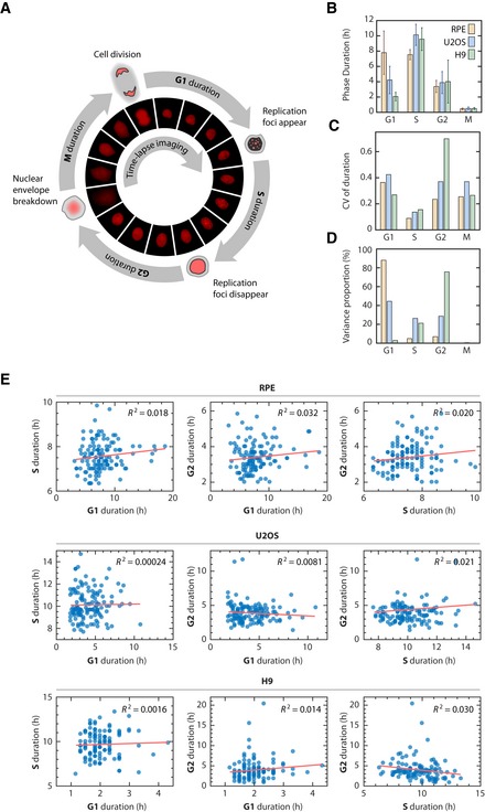
Figure 1
Variation and lack of correlation among cell cycle phase durations in single human cells
Diagramu00a0of the cell cycle composed of G1, S, G2, and M phases (not to scale). Phase durations were quantified by timeu2010lapse fluorescence microscopy using a PCNAu2010mCherry reporter to identif...
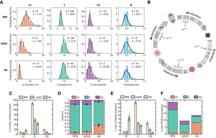
Figure 2
Erlang model of cell cycle progression
Distributions of cell cycle phase durations for RPE, U2OS, and H9 cells using singleu2010cell measurements of phase duration reported in Fig 1 . Black curves represent fits to Erlang distribution. Erl...
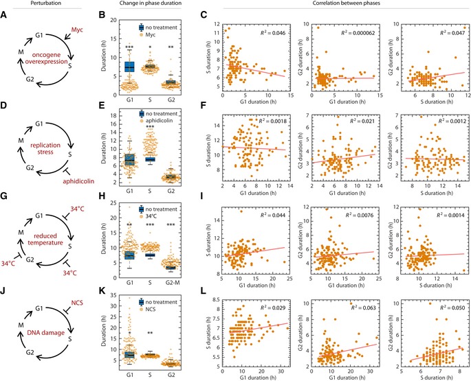
Figure 3
Lack of coupling among cell cycle phases under perturbation
Schematic of shortening G1 by myc overexpression. RPE cells infected with retrovirus harboring a tamoxifenu2010inducible myc overexpression construct. Shift in phase durations of RPE cells overexpress...
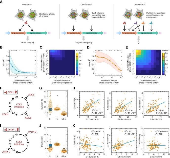
Figure 4
A model for heritable factors governing the rate of cell cycle phase progression
Alternative models for inheritance of molecular factors governing the durations of cell cycle phases. Simulation of the u201cstrength of couplingu201d as a function of the number of unique phaseu2010c...
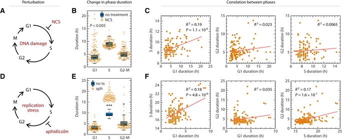
Figure 5
Stressu2010induced coupling of cell cycle phases in a cancer cell line
Schematic of prolonging G1 by DNA damage using NCS. Asynchronously proliferating U2OS mother cells were treated with 100u00a0ng/ml NCS, and their daughter cells were analyzed for a full cell cycle. Sh...
Figure images are served from the NIH/NLM PubMed Central Open Access Subset or Europe PMC; copyright remains with the publishers and authors.
💬 Discussion
0 commentsNo comments yet. Be the first to start a discussion!
Leave a Comment