Abstract
The ability to shift between repetitive and goal-directed actions is a hallmark of cognitive control. Previous studies have reported that adaptive shifts in behavior are accompanied by changes of neural activity in frontal cortex. However, neural and behavioral adaptations can occur at multiple time scales, and their relationship remains poorly defined. Here we developed an adaptive sensorimotor decision-making task for head-fixed mice, requiring them to shift flexibly between multiple auditory-motor mappings. Two-photon calcium imaging of secondary motor cortex (M2) revealed different ensemble activity states for each mapping. When adapting to a conditional mapping, transitions in ensemble activity were abrupt and occurred before the recovery of behavioral performance. By contrast, gradual and delayed transitions accompanied shifts toward repetitive responding. These results demonstrate distinct ensemble signatures associated with the start versus end of sensory-guided behavior and suggest that M2 leads in engaging goal-directed response strategies that require sensorimotor associations.
🔬 Techniques
💻 Software
✨ Fluorophores
🧪 Sample Preparation
🏭 Microscope Brands
🧪 Reagent Suppliers
🔴 Lasers
📷 Detectors
💻 Software Details
🏛️ Research Organizations (ROR)
Affiliated research institutions:
📋 Methods
Animals
Adult male mice with C57BL/6J genetic background were used. Mice were housed in groups of 3 – 5, in 12h/12h light-dark cycle (lights off at 7PM), and most experiments were performed in late afternoons and evenings (4PM – midnight). At the start of experiments, mice were P51 – 117. No statistical tests were used to pre-determine sample sizes, but sample sizes for this study are similar to those generally employed in the field. All experimental procedures were approved by the Institutional Animal Care and Use Committee, Yale University.
Surgery
Mice underwent two surgeries. For each surgery, the mouse was anesthetized with 2% isoflurane in oxygen during induction, then lowered to 1 – 1.5% for the remainder of the surgery. The mouse was placed over a water-circulating heating pad (TP-700, Gaymar Stryker) in a stereotaxic frame (David Kopf Instruments). Pre-operatively, the mouse was injected with carprofen (5 mg/kg, s.c.; #024751, Butler Animal Health) and dexamethasone (3 mg/kg, s.c.; Dexaject SP, #002459, Henry Schein Animal Health). Post-operatively, the mouse was injected with carprofen immediately after surgery (5 mg/kg, s.c.) and each day for 3 days following (5 mg/kg, s.c.). For the first surgery, an incision was made to expose the skull. Based on stereotaxic coordinates, the center location of the mouse secondary motor cortex (M2; AP = 1.5 mm, ML = 0.5 mm; relative to bregma) was marked in the right hemisphere. In other experiments, we targeted the anterior-lateral motor cortex 37 (ALM; AP = 2.5 mm, ML = 1.5 mm) or the primary visual cortex (V1; AP = −3.8 mm, ML = 2 mm) on the right hemisphere. A stainless steel head plate (eMachineshop.com) was affixed to the skull with Metabond (C&B, Parkell, Inc.), and a thin layer of clear Metabond was then applied to cover the entire skull. Mice were given at least 1 week to recover prior to behavioral training. Head plate-implanted mice were then trained on behavioral tasks (see below). Once a mouse reached a performance criterion of >90% correct rate on three consecutive days and was ready for imaging experiments, a second surgery was performed under anesthesia. Using a dental drill, a 3 mm-diameter craniotomy was made at the targeted location, which had been marked previously and remained visible through the Metabond. Dura was left intact, and was irrigated with artificial cerebrospinal fluid (ACSF, in mM: 5 KCl, 5 HEPES, 135 NaCl, 1MgCl2, 1.8 CaCl2; pH 7.3). Using a glass micropipette attached to a microinjection system (Nanoject II, Drummond), 32 – 46 nL of AAV1-Syn-GCaMP6s-WPRE-SV40 (5 x 10 13 titer; UPenn Vector Core) was injected at a depth of 400 μm below dura at each of 4 locations, vertices of a 200 μm-wide square centered at the targeted cortical region. The glass micropipette was left in place for 5 min after injection to reduce backflow. A drop of warmed agar (1.2% in ACSF, Type III-A, High EEO, A9793, Sigma-Aldrich) was then applied to the cortical surface. A two-layer glass window was fabricated by first etching out a 2-mm diameter circle from #0 thickness glass cover slip, then bonding with UV-activated polymer (61, Norland Optical Adhesive) to a #1 thickness, 3-mm diameter round glass cover slip (64-0720 CS-3R, Warner Instruments). This glass window was then placed against the cortical surface. While applying light pressure, super glue was added to the rim to attach the glass to the skull and Metabond. Mice were again given at least 1 week to recover before resuming behavioral training. Imaging experiments would begin when behavioral performance criterion was reached. Eight out of eleven mice went through this procedure involving two surgeries. For the remaining three mice, the head plate implant, viral injection, and window implant procedures were performed in the same surgery before behavioral training.
Show full methods section
Animals
Adult male mice with C57BL/6J genetic background were used. Mice were housed in groups of 3 – 5, in 12h/12h light-dark cycle (lights off at 7PM), and most experiments were performed in late afternoons and evenings (4PM – midnight). At the start of experiments, mice were P51 – 117. No statistical tests were used to pre-determine sample sizes, but sample sizes for this study are similar to those generally employed in the field. All experimental procedures were approved by the Institutional Animal Care and Use Committee, Yale University.
Surgery
Mice underwent two surgeries. For each surgery, the mouse was anesthetized with 2% isoflurane in oxygen during induction, then lowered to 1 – 1.5% for the remainder of the surgery. The mouse was placed over a water-circulating heating pad (TP-700, Gaymar Stryker) in a stereotaxic frame (David Kopf Instruments). Pre-operatively, the mouse was injected with carprofen (5 mg/kg, s.c.; #024751, Butler Animal Health) and dexamethasone (3 mg/kg, s.c.; Dexaject SP, #002459, Henry Schein Animal Health). Post-operatively, the mouse was injected with carprofen immediately after surgery (5 mg/kg, s.c.) and each day for 3 days following (5 mg/kg, s.c.). For the first surgery, an incision was made to expose the skull. Based on stereotaxic coordinates, the center location of the mouse secondary motor cortex (M2; AP = 1.5 mm, ML = 0.5 mm; relative to bregma) was marked in the right hemisphere. In other experiments, we targeted the anterior-lateral motor cortex 37 (ALM; AP = 2.5 mm, ML = 1.5 mm) or the primary visual cortex (V1; AP = −3.8 mm, ML = 2 mm) on the right hemisphere. A stainless steel head plate (eMachineshop.com) was affixed to the skull with Metabond (C&B, Parkell, Inc.), and a thin layer of clear Metabond was then applied to cover the entire skull. Mice were given at least 1 week to recover prior to behavioral training. Head plate-implanted mice were then trained on behavioral tasks (see below). Once a mouse reached a performance criterion of >90% correct rate on three consecutive days and was ready for imaging experiments, a second surgery was performed under anesthesia. Using a dental drill, a 3 mm-diameter craniotomy was made at the targeted location, which had been marked previously and remained visible through the Metabond. Dura was left intact, and was irrigated with artificial cerebrospinal fluid (ACSF, in mM: 5 KCl, 5 HEPES, 135 NaCl, 1MgCl2, 1.8 CaCl2; pH 7.3). Using a glass micropipette attached to a microinjection system (Nanoject II, Drummond), 32 – 46 nL of AAV1-Syn-GCaMP6s-WPRE-SV40 (5 x 10 13 titer; UPenn Vector Core) was injected at a depth of 400 μm below dura at each of 4 locations, vertices of a 200 μm-wide square centered at the targeted cortical region. The glass micropipette was left in place for 5 min after injection to reduce backflow. A drop of warmed agar (1.2% in ACSF, Type III-A, High EEO, A9793, Sigma-Aldrich) was then applied to the cortical surface. A two-layer glass window was fabricated by first etching out a 2-mm diameter circle from #0 thickness glass cover slip, then bonding with UV-activated polymer (61, Norland Optical Adhesive) to a #1 thickness, 3-mm diameter round glass cover slip (64-0720 CS-3R, Warner Instruments). This glass window was then placed against the cortical surface. While applying light pressure, super glue was added to the rim to attach the glass to the skull and Metabond. Mice were again given at least 1 week to recover before resuming behavioral training. Imaging experiments would begin when behavioral performance criterion was reached. Eight out of eleven mice went through this procedure involving two surgeries. For the remaining three mice, the head plate implant, viral injection, and window implant procedures were performed in the same surgery before behavioral training.
Behavioral setup
For head-fixed mouse behavior, we used a training apparatus that has two lick ports, thus enabling two alternative choices. The use of two lick ports was inspired by another study 37 . Two metal screws were used to affix the head plate of the mouse onto a stainless steel mount. The mouse was then restrained inside an acrylic tube, which restricted gross body movements but allowed postural adjustments. The lick ports were fabricated from stainless steel 20-gauge needles, which were positioned at 90 and 270 degrees with respect to the mouse’s head orientation, and held in place by a 3D-printed plastic part mounted on a micromanipulator for fine positional adjustment. Water was delivered at the ports by gravity feed and the liquid volume was controlled by pneumatic valves (EV-2-24, Clippard), calibrated with an intravenous dripper to deliver ~2 μL per pulse. A battery-operated touch detector circuit signaled when the mouse’s tongue contacted a lick port. Auditory stimuli were played through computer speakers placed directly in front of the animal. The intensity of the auditory stimuli was calibrated to ~85 dB peak amplitude. Water delivery, lick detection, and sound presentation were connected to a desktop computer via a data acquisition board (USB-201, Measurement Computing). Presentation software (Neurobehavioral Systems) controlled the entire behavioral system. An infrared webcam was used to monitor the animal while in the rig. Behavioral training was performed inside the closed compartment of an audio-visual cart that was dark and soundproofed with acoustic foams (5692T49, McMaster-Carr). For imaging, mice were tested using a replica of the behavioral training setup under a two-photon microscope. Adaptive decision-making task To motivate participation in the task, water consumption was restricted to behavioral sessions. Mice were trained for 1 session per day, 6 days a week. On the non-training day, water was provided ad libitum in the home cage for 15 min. The mice were trained through four phases to shape their behavior. Phase one (~2 days): mice were habituated to head fixation in the behavior box, and trained to lick either one of the two ports for water reward. Mice were advanced to the next phase when they made >100 responses in a session. Phase two (~2 days), mice were trained to sample both ports. Here, mice were required to lick the left port to obtain water rewards three times, followed by the right port for the next three rewards, and so on. Mice were advanced to the next phase when they made >100 correct responses in a session. Phase three (>15 days), animals underwent training for two-choice auditory discrimination. One of two auditory cues was presented to begin each trial: a 2 s-long train of 0.5 s-long logarithmic frequency modulated sweeps from 5-to-15 kHz (“upsweep”) or from 15-to-5 kHz (“downsweep”). The stimuli were interleaved randomly from trial to trial. At 0.5 s following the onset of the auditory cue, a response window would open lasting for a maximum duration of 2 s. The animal's first lick within this response window was registered as its response for the trial. All other licks were logged but had no consequences. Once a response was recorded, playback of the auditory cue was terminated. A correct response, i.e. a left lick for upsweep or a right lick for downsweep, resulted in immediate delivery of 2 μL of water from the corresponding port. The next trial would begin 6 s following response. Incorrect responses resulted in 2 s of white noise presentation, with the next trial beginning 4 s later. Each trial had a total duration within a range from 7.5 to 9 s. Animals were allowed to perform trials until satiated (20 consecutive misses), typically after ~60 minutes. Training continued daily until a correct rate of >90% was attained for 3 consecutive days. For imaging experiments, mice were then trained under the two-photon microscope (with laser turned off) for habituation to the recording setup. All the mice were able to discriminate at >90% correct rate after 1–3 days of re-training. Finally, mice were tested on the adaptive decision-making task. The task always began with a sound block (S) indistinguishable from the two-choice auditory discrimination task. However, once the mouse reached a performance criterion of >85% correct for the last 20 trials, the stimulus-response-outcome contingencies would change from sound- to action-guided trials. In action-guided trials, task structure was identical to sound-guided trials. However, the correct response became fixed to one response direction, e.g. always left, regardless of the stimulus identity. No cue signaled the change in contingencies. When the mouse reached performance criterion again, another block switch would occur. A sound block was always followed by an action block, and vice versa. The second block was randomly chosen for each experiment to be action-left (AL) or action-right (AR). However, once the first action block was chosen, the block sequence became fixed for the remainder of the session. Therefore, the sequence of blocks could be one of two possibilities: (S-AL-S-AR-S-AL-S-AR…) or (S-AR-S-AL-S-AR-S-AL-…). Each session was terminated after 20 consecutive misses (trials with no response). Mice typically performed the adaptive decision-making task for 60 – 90 min. Following each adaptive decision-making test, mice resumed daily two-choice auditory discrimination until the next recording session, up to a maximum of seven adaptive decision-making tests. Our behavioral paradigm consists of blocks of trials that require the animal to shift between conditional and non-conditional approaches to action selection. In principle, mice may solve this task by ignoring sensory information completely during action blocks. However, the temporally structured lick rates during action blocks ( Fig. 1e ) strongly suggest use of the stimulus for gating lick responses. Our task has similarities with other paradigms that test behavioral flexibility, but there are also crucial differences. In contrast to paradigms that use a contextual cue to instruct rapid executive control on a trial-by-trial basis 9 , 10 , 39 , animals adapt on a time scale of tens of trials in our task ( Fig. 1c ). This relatively slow rate of adaptation is akin to learning during arbitrary visuomotor mapping, where the animal’s basis for action selection is updated gradually based on reward feedback 7 , 40 . Our task also differs from other strategy- or set-shifting tasks for rodents 12 , 41 because non-spatial stimuli were used to probe arbitrary sensorimotor associations that do not conform to classical definitions of exemplars or sets. Furthermore, analysis of the types of errors made during training suggests that mice perform two-choice auditory discrimination in part by suppressing a prepotent tendency to repeat a rewarded choice. Action trials could thus be considered a natural strategy to the animal, whereas sound-guided trials require weeks of training to achieve high performance. Therefore, one caveat for our task is that animals are likely to have different degrees of learned and intrinsic familiarity for sound versus action trials.
Two-photon calcium imaging
The two-photon microscope (Movable Objective Microscope, Sutter Instrument) was controlled using ScanImage software 51 . The excitation source was an ultrafast laser (Chameleon Ultra II, Coherent). Excitation intensity was controlled by a Pockels cell (350-80-LA-02, Conoptics) and focused onto the sample with a 20x, N.A. 0.95 water immersion objective (Olympus). The time-averaged excitation laser intensity was 90–100 mW after the objective. To image fluorescence transients from GCaMP6s-expressing neurons, excitation wavelength was set at 920 nm, and emission was collected from 475 – 550 nm with a GaAsP photomultiplier tube. Time-lapse images were acquired at a resolution of 256 x 256 pixels and a frame rate of 3.62 Hz using bidirectional scanning. To synchronize behavior with imaging, a TTL pulse was sent at the beginning of each trial from the data acquisition board of the behavioral system to the imaging system to act as an external trigger for initiating image acquisition. Inactivation Mice were implanted with a head plate. The locations of M2 were marked on both hemispheres (AP = 1.5 mm, ML = 0.5 mm), and then covered with a thin layer of clear Metabond. Mice were then trained as described above, in preparation for the adaptive decision-making test. Craniotomies were performed at the marked locations. Using a glass micropipette attached to a microinjection system (Nanoject II, Drummond), ACSF, with or without muscimol (5 mM, 46 nL per hemisphere; cat. #195336, MP Biomedical), was injected at a depth of 400 μm into M2 of both hemispheres. Behavioral testing began 1–3 hr following injection. The same mice were tested after saline and muscimol treatments on consecutive days in a counter-balanced design, with no blinding. The mice were randomized to receive either saline or muscimol first in an alternating manner depending on the order in which they reached the behavioral performance criterion. Twelve mice were allocated for this experiment; however, one was excluded due to equipment malfunction during testing.
Histology
Following experiments, mice underwent transcardial perfusion with chilled formaldehyde solution (4% in phosphate-buffered saline). The brains were sectioned with a vibratome and imaged with an inverted wide-field fluorescence microscope. Analysis: behavioral data Timestamps of stimulus presentation, licks, and water delivery were logged in a text file by Presentation software (Neurobehavioral Systems, Inc.). Scripts were written in MATLAB to parse the log files. For the adaptive decision-making task, a perseverative error was defined as an incorrect response that would have been correct according to the last trial block’s contingencies. For example, during an action-left block, the stimulus-response pairings of upsweep-left lick and downsweep-left lick would be “correct”. Downsweep-right lick would be a “perseverative error”, because this stimulus-response pairing would have been correct in the preceding sound-guided block. The remaining possible stimulus-response pairing, upsweep-right lick, would be classified as an “other error”. The number of trials performed included all correct and error trials, but excluded the miss trials when the mouse failed to lick within the response window. Miss trials typically occurred near the end of the session when the mouse was satiated. Trials-to-criterion was defined as the number of trials performed in a certain trial block before reaching a performance criterion of 85% correct for the last 20 trials. Therefore, the minimum value of this quantity is 20. Mean trials to criterion for each session was calculated excluding the first sound block, because contingency switches have not yet begun. Mean blocks per 100 trials, mean perseverative errors per block, and mean other errors per block were calculated excluding the last block (i.e. trials after the last block switch). For analysis, we often compared pre-switch and post-switch conditions, which were defined as the 20 trials prior to or following a block switch. The first lick time was defined as the time of the first lick after sound onset for each trial, which may occur prior to the start of the response window. The first lick time is thus a sum of the reaction time and movement time. For this measurement, we excluded trials in which the mouse licked within 0.5 s before cue onset, in which case the first lick may represent the continuation of a spontaneous lick bout rather than a reaction to the stimulus. Analysis: imaging data Time-lapse fluorescence images were corrected for x-y motion using the TurboReg plug-in for ImageJ (NIH). We wrote a GUI in MATLAB to select cell bodies as regions of interest (ROIs). Values of pixels within an ROI were averaged to generate F C (t). For each cell, we estimated the neuropil signal by drawing a doughnut 52 , by approximating the ROI area as a circle to estimate a radius r , then creating an annulus-shaped neuropil area with inner and outer diameters of 2 r and 3 r . This neuropil area excluded pixels if they were part of the ROI of another cell body. Values of pixels within the annulus-shaped neuropil area were averaged to generate F N (t) . To subtract the neuropil signal, we calculated F(t) = F C (t) - α F N (t) , where α is a correction factor ranging from 0.2 – 0.6. The value of α was calibrated for each experiment to avoid over-correction, by making sure that F(t) > 0 for each cell. For each ROI, the fractional change in fluorescence, Δ F / F(t) , was calculated as: Δ F F ( t ) = F ( t ) - F o ( t ) F o ( t ) , where F o (t) is the baseline fluorescence as a function of time. To estimate baseline, we first obtained F image (t) , the mean pixel intensity for the entire 256 pixel x 256 pixel field of view as a function of time. F o (t) was then calculated as: F o ( t ) = F ∗ × F o , image ( t ) F o , image ∗ , where F o,image (t) is the 10 th percentile of F image (t) within a sliding window of 10 minute duration. F* and F* o,image are the 10 th percentile of F(t) and F o,image (t) within the first 10 minutes of the session, respectively. We verified that F 0,image (t)/F* 0,image does not vary with specific choices or rule blocks, and thus serves the purpose of compensating for slow, full-field signal drifts due to non-physiological sources. We have repeated the ensemble analyses with two other methods for calculating baseline. One, estimating F o (t) using the 10 th percentile of F(t) , on a per-cell basis, with a moving window of 10 minute duration. Two, estimating F o (t) using the 10 th percentile of F(t) from the entire session, i.e. without a moving window. These different ways to estimate baseline led to qualitatively similar results for all the ensemble analyses. Analysis: task-related activity and choice encoding To calculate trial-averaged fluorescence transients, we created time bins that were 0.5 s wide, and then assigned each ΔF/F(t) value at a particular time t to the corresponding time bin relative to the animal’s response. The binned ΔF/F(t) values were averaged to obtain trial-averaged ΔF/F . To estimate uncertainty of the trial-averaged ΔF/F , a bootstrap analysis was performed by drawing fluorescence transients per trial, with replacement, up to the same number used to construct the trial average. The median and 95% confidence intervals of trial-averaged ΔF/F were estimated from 1000 iterations of this bootstrap analysis. To quantify choice encoding, we performed multiple linear regression analysis on the ΔF/F(t) of each cell using the following equation: Δ F F ( t ) = a 0 + a 1 C ( n ) + a 2 C ( n - 1 ) + a 3 C ( n ) C ( n - 1 ) + a 4 C ( n - 2 ) + ε ( t ) , where C(n) was the choice of current trial, C(n-1) was the choice of prior trial, C(n-2) was the choice two trials ago, ε(t) was the error term and a ’s were regression coefficients. We coded a choice of left as 1 and right as −1. We used a non-overlapping 0.5 s-long moving window with step size of 0.5 s. A cell was deemed to encode one of the choice parameters or interaction if p < 0.01 for the corresponding regression coefficient. To avoid confounds from rule and reward signals, we analyzed only sound-guided trials in which R(n) = 1 (outcome of current trial = reward) and R(n-1) = 1 (outcome of prior trial = reward). We did not analyze action trials, because parameters such as C(n) and C(n-1) were highly correlated by virtue of the task structure, obviating a simple interpretation of the analysis. Analysis: neural circuit trajectories Scripts for the ensemble analysis were written in MATLAB, and are available upon request. For state-space analysis, we used demixed principal component analysis 36 (dPCA). To prepare the imaging data for dPCA, ΔF/F(t) for each cell for each trial was aligned in time, from 0 to 6 s from the time of the response in that trial. We have tried numerous other time windows and found similar results. This alignment led to an array with dimensions = cells x time x trials. Using this array, we averaged across 4 trial types: C(n) = 1, R(n) = 1, pre-switch sound trials; C(n) = −1, R(n) = 1, pre-switch sound trials; C(n) = 1, R(n) = 1, pre-switch action trials; C(n) = −1, R(n) = 1, pre-switch action trials. This trial-averaged array (cells x time x 4) was input into the dPCA algorithm 36 to demix time- and task-dependent variances and obtain principal components (PCs). To calculate neuronal circuit trajectories, single-trial or trial-averaged ΔF/F were projected onto the first three PCs. To characterize similarities between the neuronal circuit trajectories across blocks, we calculated the neuronal circuit trajectory for each block by using the trial-averaged fluorescence across the 20 trials pre-switch. The similarity between a pair of trajectories was quantified by calculating the mean of the Euclidean distances between the trajectories at matching time points in state-space. In order to compare between different experiments, this distance was normalized for each experiment: the Euclidean distances were divided by the spread of all population vectors, calculated as the root mean square of distances between all population vectors and the centroid of the vectors. To quantify how the neuronal circuit trajectories evolve on a trial-to-trial basis, we used the Mahalanobis distance, which is a measure of distance between one point and another collection of points. We defined the origin as the 20 trials preceding a block switch, and the destination as the 20 trials preceding the next block switch. We were interested in the relative separation between the origin, an individual trial that occurred in between, and the destination. Therefore, for each time point of a trial, we calculated Mahalanobis distances, d origin (t) and d dest (t) , from the individual trial (1 three-dimensional value) to the origin and destination respectively (20 three-dimensional values). The d origin (n) and d dest (n) for each individual trial is the median of d origin (t) and d dest (t) of the ~30 time points within a trial. To estimate the location of an individual trial relative to the origin and destination, we calculated the ratio of Mahalanobis distances, d origin (n) / (d origin (n) + d dest (n)) . For the Mahalanobis distance ratios, which are a function of trial number from switch, we fitted with a logistic function, f ( x ) = L 1 + e - k ( x - x o ) + L min , where x 0 is the midpoint trial, k is the steepness, L is the range, and L min is the minimum value. The parameter L min is not fitted, but rather estimated for each transition by calculating the mean of Mahalanobis distance ratio using trials −5 to −1 from switch. We fitted every neural ensemble transition using this method, but excluded those in which the midpoint trial x 0 < −5 or x 0 > 200, indicating a poor fit. Based on this criterion, we excluded none (0/33) of the action-to-sound shifts and 8% (3/38) of the sound-to-action shifts in our analysis of M2 neural ensembles. For analysis of the ALM data set, we excluded 8% (2/26) of the action-to-sound shifts and 3% (1/32) of the sound-to-action shifts. When comparing behavioral and neural transitions, we defined ‘behavioral transition trial’ as the trial to criterion (85% correct for 20 trials) subtracted by 20, i.e. the first of the sequence of 20 trials leading to block switch. The ‘neural transition trial’ was defined as the trial when the first term of the logistic fit of Mahalanobis distance ratios reached a value of 75% L . That is, the trial x that satisfies this equation: 0.75 L = L 1 + e - k ( x - x o ) . This definition is arbitrary; it is unknown how much the population activity pattern must resemble the final pre-switch ensemble state in order to qualify as a ‘transition’. Therefore, in another analysis we first fitted each neural transition with the logistic function, and identified the behavioral trial corresponding to each 5% L step of neural transition from 10 to 90% L . We then calculated the mean hit and error rates at those corresponding behavioral trials, thus plotting the relationship between behavioral performance and neural transition without explicitly defining a transition trial. Analysis: decoding To determine how well ensemble dynamics could be used to predict trial type, we first selected those imaging frames that occurred between 0 to 6 s from time of response out of the frame-by-frame imaging data (i.e., ΔF/F(t) ). We then projected these ΔF/F(t) onto the PCs deduced from dPCA to obtain population activity vectors. This procedure reduced the dimensionality of our data from (frames × cells) to (frames × 3). Each population activity vector in this analysis came from one of four possible trial types: R(n) =1, pre-switch sound trials; R(n) =1, pre-switch action-left trials; R(n) =1, pre-switch action-right trials; other trial types were not considered for the decoding analysis. Using a randomly chosen fraction (80%) of the population activity vectors, we constructed a classifier based on linear discriminant analysis, using Mahalanobis distances with stratified covariance estimates (the “classify” function in MATLAB with “Mahalanobis” option). We then tested the performance of this classifier on the remaining 20% of the population activity vectors, comparing the classification results with actual trial types. This five-fold cross-validation process was repeated 1,000 times to obtain a median estimate of classifier accuracy. To investigate decoding accuracy across time, the timing information of each population activity vector relative to the time of response in each trial was retained. We then ran a separate decoding analysis on the population activity vectors measured during each time period, using a non-overlapping sliding window with duration of 0.28 s and step size of 0.28 s. This window duration is the inverse of frame rate, which was 3.6 Hz. To decode from single-cell activity, ΔF/F(t) of each cell was used instead of population activity vectors as inputs to construct the classifier.
Statistics
Statistical tests were performed in MATLAB, and are indicated in the main text or figure legends. Briefly, a Wilcoxon signed-rank test was used for all two-sample, paired comparisons. For two-sample, unpaired comparisons, a Wilcoxon rank-sum test was used. Paired t-tests were used for bin-wise analysis of lick rates. For quantification of choice signals as a function of time, multiple linear regression was first performed as detailed above; a binomial test was then applied to the proportion of cells significantly encoding choice within each time-bin. For ensemble decoding analyses, mean classification accuracy was tested against chance level using a one-sample t-test. For t-tests, the sampling distribution of the mean was assumed to be normal, but this was not formally tested. All t-tests were two-tailed. A statistics checklist is available in the Supplementary Materials .
Code availability
The custom MATLAB code used for this study is available upon request.
Data availability
The data that support the findings of this study are available from the corresponding author upon request.
Supplementary Material 1 2 3
📊 Figures
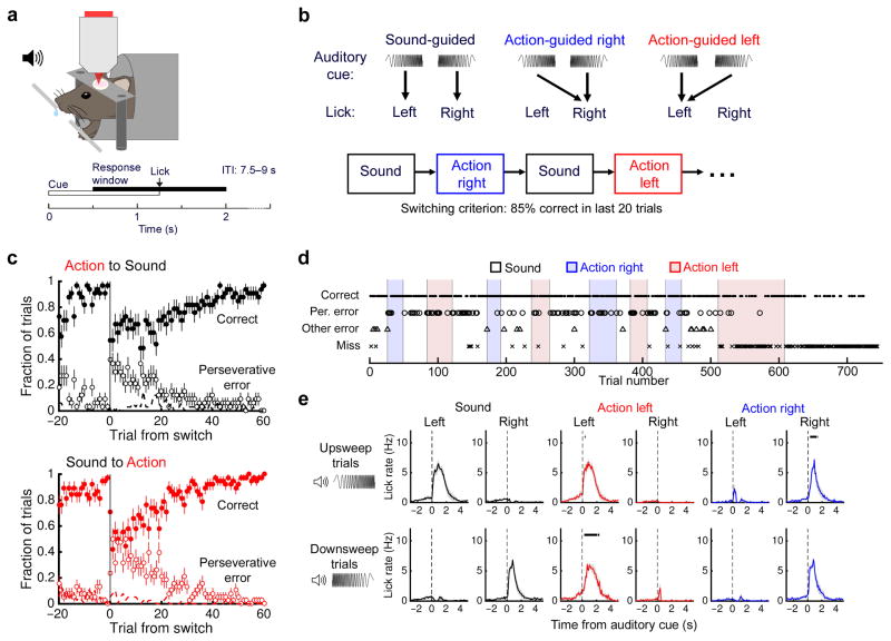
Figure 1
Behavioral performance of head-fixed mice in an adaptive sensorimotor decision-making task
( a ) Schematic of experiment. Each trial begins with an auditory cue.nA response window starts 0.5 s after cue onset, during which the first lick isnrecorded as the response for that trial. Water rew...
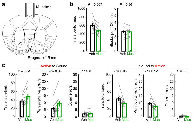
Figure 2
Bilateral inactivation of secondary motor cortex impairs adjustment to sound-guided trials
( a ) Schematic of experiment. ( b ) Task performance after bilateral infusion of saline vehiclen(Veh) or muscimol (Mus) into M2 ( c ) Effects of muscimol infusion on action-to-sound andnsound-to-acti...
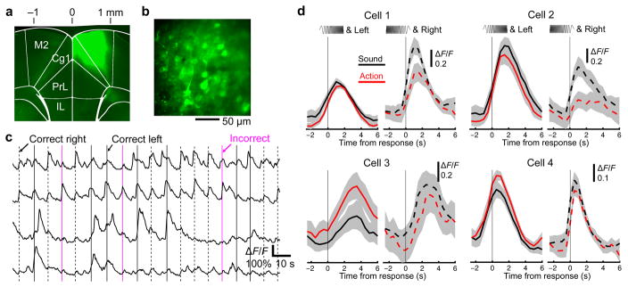
Figure 3
Two-photon calcium imaging of task-related activity in secondary motor cortex
( a ) Example post hoc and ( b ) in vivo two-photon images of GCaMP6s-expressingnneurons in layer 2/3 of M2. ( c ) Fractional fluorescence changes ( u0394F/F )nin example M2 neurons during performance...
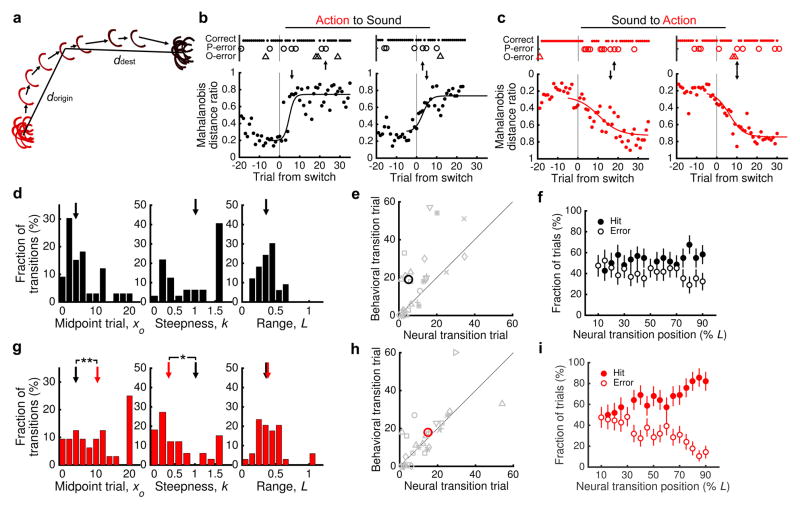
Figure 4
Transitions in ensemble activity occur earlier and are more abrupt following switch to sound-guided trials
( a ) A schematic illustrating ensemble activity dynamics around anblock switch. Each curved line represents a single-trial neural trajectoryndeduced from calcium imaging data. When the contingencies ...
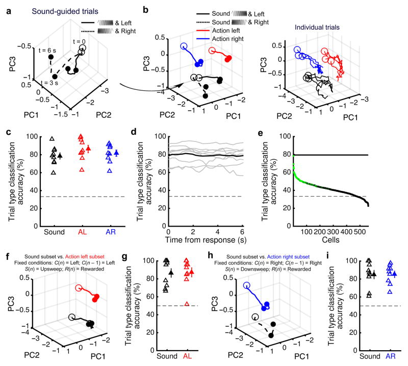
Figure 5
Multiple strategies are associated with distinct population activity patterns
( a ) Neuronal circuit trajectories for an ensemble of 56nsimultaneously imaged cells in one experiment. Trajectories were determined fromntrial-averaged u0394F/F for 44 correct left (dotted line)nand...
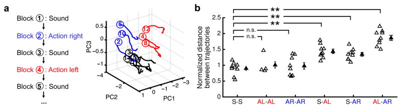
Figure 6
M2 ensembles revisit previous activity patterns upon re-exposure to corresponding trial-type
( a ) Neural circuit trajectories, calculated from trial-averaged u0394F/F for each trial block during one behavioralnsession. Circled numbers denote temporal order in which trial blocks werenpresente...
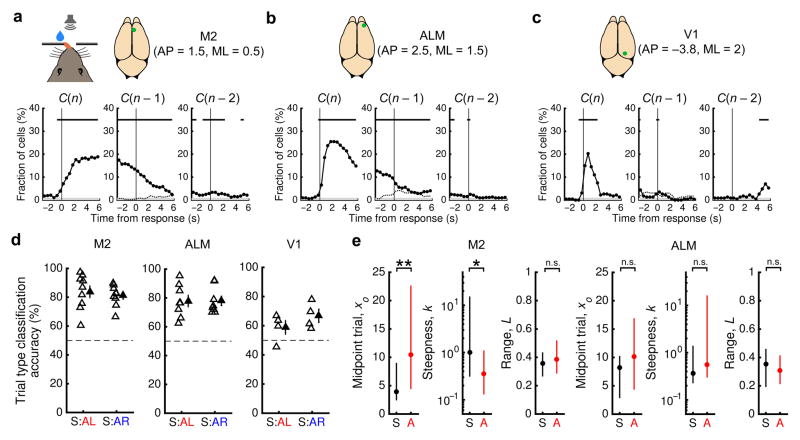
Figure 7
Comparison between neural activity patterns in M2, ALM, and V1 during flexible sensorimotor behavior
( a ) Multiple linear regression analysis was used to evaluate thenfraction of 562 M2 neurons encoding choice signals as a function of time.nRegression was performed with a moving window (duration = 0...
Figure images are served from the NIH/NLM PubMed Central Open Access Subset or Europe PMC; copyright remains with the publishers and authors.
💬 Discussion
0 commentsNo comments yet. Be the first to start a discussion!
Leave a Comment