Abstract
Abstract Bacteria have evolved macromolecular machineries that secrete effectors and toxins to survive and thrive in diverse environments. The type VI secretion system (T6SS) is a contractile machine that is related to Myoviridae phages. It is composed of a phage tail‐like structure inserted in the bacterial cell envelope by a membrane complex (MC) comprising the TssJ, TssL and TssM proteins. We previously reported the low‐resolution negative‐stain electron microscopy structure of the enteroaggregative Escherichia coli MC and proposed a rotational 5‐fold symmetry with a TssJ:TssL:TssM stoichiometry of 2:2:2. Here, cryo‐electron tomography analyses of the T6SS MC confirm the 5‐fold symmetry in situ and identify the regions of the structure that insert into the bacterial membranes. A high‐resolution model obtained by single‐particle cryo‐electron microscopy highlights new features: five additional copies of TssJ, yielding a TssJ:TssL:TssM stoichiometry of 3:2:2, an 11‐residue loop in TssM, protruding inside the lumen of the MC and constituting a functionally important periplasmic gate, and hinge regions. Based on these data, we propose an updated model on MC structure and dynamics during T6SS assembly and function.
🔬 Techniques
🔭 Microscopes
🧬 Organisms
💻 Software
✨ Fluorophores
🧪 Sample Preparation
🔬 Cell Lines
🏭 Microscope Brands
🧪 Reagent Suppliers
📷 Detectors
💻 Software Details
💾 Data Repositories
🏛️ Research Organizations (ROR)
Affiliated research institutions:
📋 Methods
Strains and media
Strains used in this study are listed in Appendix Table S1 . The E. coli K‐12 W3110 bearing the pUA66‐ rrnB vector (Kan R and GFP + , Zaslaver et al , 2006 ) was used as recipient for antibacterial competition assays. Strains were routinely grown in lysogeny broth (LB)‐rich medium or in Sci‐1‐inducing medium (SIM; M9 minimal medium, glycerol 0.2%, vitamin B1 1 μg/ml, casamino acids 100 mg/ml, LB 10%, supplemented or not with bacto agar 1.5%; Brunet et al , 2011 ) with shaking at 37°C. Strain construction tssM and tssJ point mutations were engineered at the native locus on the chromosome by allelic replacement using the pKO3 suicide vector (Link et al , 1997 ) into the enteroaggregative E. coli 17‐2 strain. Briefly, 17‐2 WT strain was transformed with a pKO3 plasmid in which a fragment of the tssM or tssJ gene carrying the point mutations has been cloned (see below). Insertion of the plasmid into the chromosome was selected on chloramphenicol plates at 42°C. Plasmid sequences removal was then selected on 5% sucrose plates without antibiotic, and tssM point mutation recombinant strains were screened by PCR and confirmed by DNA sequencing (Eurofins, MWG). Chromosomal fluorescent reporter insertions into the enteroaggregative E. coli 17‐2 strain mutated in tssM or tssJ were achieved by using a modified one‐step inactivation procedure (Datsenko & Wanner, 2000 ) as previously described (Aschtgen et al , 2008 ) using plasmid pKOBEG (Chaveroche et al , 2000 ). Briefly, a kanamycin cassette was amplified from plasmid pKD4 using oligonucleotide pairs carrying 5′ 50‐nucleotide extensions homologous to regions adjacent to the gene to be deleted. After electroporation of 600 ng of column‐purified PCR product, kanamycin‐resistant clones were selected and verified by colony PCR. The kanamycin cassette, inserted at the gene locus on the bacterial chromosome, was then excised using plasmid pCP20, leaving an FRT scars. Gene deletions were confirmed by colony PCR and sequencing. Fluorescence microscopy, image treatment and analyses Fluorescence microscopy experiments were performed as described (Brunet et al , 2013 ; Zoued et al , 2013 ). Briefly, cells were grown overnight in LB medium and diluted to A 600 nm ~0.04 in SIM. Exponentially growing cells ( A 600 nm ~0.8–1) were harvested, washed in phosphate‐buffered saline buffer (PBS), resuspended in PBS to A 600 nm ~50, spotted on a 1.5% agarose pad and covered with a cover slip. Fluorescence micrographs were captured using AxioImager M2 microscope (Zeiss) equipped with an OrcaR2 digital camera (Hamamatsu). For time‐lapse fluorescence microscopy, images were recorded with a Nikon Eclipse Ti microscope equipped with an Orca‐Flash 4.0 LT digital camera (Hamamatsu) and a perfect focus system (PFS) to automatically maintain focus so that the point of interest within a specimen is always kept in sharp focus at all times despite mechanical or thermal perturbations. Fluorescence images were acquired with a minimal exposure time to reduce bleaching and phototoxicity effects, typically 200 ms for TssB sfGFP and 300 ms for sfGFP TssM. For image treatment, noise and background were reduced using the “Subtract Background” (20 pixels Rolling Ball) and Band plugins of imageJ (Schneider et al , 2012 ). The sfGFP foci were automatically detected using the microbeJ plugin (Ducret et al , 2016 ). Floating bars representing the number of detected foci for each strain were made using GraphPad ( https://www.graphpad.com ). Microscopy analyses were performed at least three times, each in technical triplicate, and a representative experiment is shown.
Show full methods section
Strains and media
Strains used in this study are listed in Appendix Table S1 . The E. coli K‐12 W3110 bearing the pUA66‐ rrnB vector (Kan R and GFP + , Zaslaver et al , 2006 ) was used as recipient for antibacterial competition assays. Strains were routinely grown in lysogeny broth (LB)‐rich medium or in Sci‐1‐inducing medium (SIM; M9 minimal medium, glycerol 0.2%, vitamin B1 1 μg/ml, casamino acids 100 mg/ml, LB 10%, supplemented or not with bacto agar 1.5%; Brunet et al , 2011 ) with shaking at 37°C. Strain construction tssM and tssJ point mutations were engineered at the native locus on the chromosome by allelic replacement using the pKO3 suicide vector (Link et al , 1997 ) into the enteroaggregative E. coli 17‐2 strain. Briefly, 17‐2 WT strain was transformed with a pKO3 plasmid in which a fragment of the tssM or tssJ gene carrying the point mutations has been cloned (see below). Insertion of the plasmid into the chromosome was selected on chloramphenicol plates at 42°C. Plasmid sequences removal was then selected on 5% sucrose plates without antibiotic, and tssM point mutation recombinant strains were screened by PCR and confirmed by DNA sequencing (Eurofins, MWG). Chromosomal fluorescent reporter insertions into the enteroaggregative E. coli 17‐2 strain mutated in tssM or tssJ were achieved by using a modified one‐step inactivation procedure (Datsenko & Wanner, 2000 ) as previously described (Aschtgen et al , 2008 ) using plasmid pKOBEG (Chaveroche et al , 2000 ). Briefly, a kanamycin cassette was amplified from plasmid pKD4 using oligonucleotide pairs carrying 5′ 50‐nucleotide extensions homologous to regions adjacent to the gene to be deleted. After electroporation of 600 ng of column‐purified PCR product, kanamycin‐resistant clones were selected and verified by colony PCR. The kanamycin cassette, inserted at the gene locus on the bacterial chromosome, was then excised using plasmid pCP20, leaving an FRT scars. Gene deletions were confirmed by colony PCR and sequencing. Fluorescence microscopy, image treatment and analyses Fluorescence microscopy experiments were performed as described (Brunet et al , 2013 ; Zoued et al , 2013 ). Briefly, cells were grown overnight in LB medium and diluted to A 600 nm ~0.04 in SIM. Exponentially growing cells ( A 600 nm ~0.8–1) were harvested, washed in phosphate‐buffered saline buffer (PBS), resuspended in PBS to A 600 nm ~50, spotted on a 1.5% agarose pad and covered with a cover slip. Fluorescence micrographs were captured using AxioImager M2 microscope (Zeiss) equipped with an OrcaR2 digital camera (Hamamatsu). For time‐lapse fluorescence microscopy, images were recorded with a Nikon Eclipse Ti microscope equipped with an Orca‐Flash 4.0 LT digital camera (Hamamatsu) and a perfect focus system (PFS) to automatically maintain focus so that the point of interest within a specimen is always kept in sharp focus at all times despite mechanical or thermal perturbations. Fluorescence images were acquired with a minimal exposure time to reduce bleaching and phototoxicity effects, typically 200 ms for TssB sfGFP and 300 ms for sfGFP TssM. For image treatment, noise and background were reduced using the “Subtract Background” (20 pixels Rolling Ball) and Band plugins of imageJ (Schneider et al , 2012 ). The sfGFP foci were automatically detected using the microbeJ plugin (Ducret et al , 2016 ). Floating bars representing the number of detected foci for each strain were made using GraphPad ( https://www.graphpad.com ). Microscopy analyses were performed at least three times, each in technical triplicate, and a representative experiment is shown.
Interbacterial competition assay
The antibacterial growth competition assay was performed as previously described (Flaugnatti et al , 2016 ). Wild‐type E. coli K‐12 strain W3110 bearing the pUA66‐ rrnB plasmid conferring kanamycin resistance and constitutive GFP fluorescence ( gfp gene under the control of the ribosomal rrnB promoter, Gueguen & Cascales, 2013 ) was used as recipient. Attacker and recipient cells were grown for 16 h in LB medium, diluted in SIM to allow maximal expression of the sci‐1 gene cluster (Brunet et al , 2011 ). Once the culture reached A 600 nm ~0.8, cells were harvested and normalized to A 600 nm = 0.5 in SIM. Attacker and recipient cells were mixed to a 4:1 ratio and 15‐μl drops of the mixture were spotted in triplicate onto a pre‐warmed dry SIM agar plate. After incubation for 4 h at 37°C, the bacterial spots were resuspended in LB and bacterial suspensions were normalized to A 600 nm = 0.5. For the enumeration of viable prey cells, bacterial suspensions were serially diluted and spotted onto kanamycin LB plates. The assays were performed from at least three independent cultures, with technical triplicates, and a representative technical triplicate is shown.
Protein preparation
The expression and purification of the TssJLM complex were carried out as previously described (Durand et al , 2015 ), with the exception that the cryo‐EM grids were prepared immediately after the HisTrap Elution. For the amphipole‐containing sample, the Strep‐Trap elution was incubated with amphipoles A8‐35 (Anatrace, USA) and subjected to gel filtration on a superpose 6 (GE Healthcare, UK) to remove residual detergent.
Cryo‐EM grids preparation and data acquisition C‐flat™
(CF‐2/1‐2C) grids were coated with graphene oxide as previously described (Martin et al , 2016 ). 3.5 μl of the sample at 0.2 mg/ml was loaded on the copper side and then blotted on the same side for 2 s in a Leica EM GP at 80% humidity and 4°C, before being plunge‐frozen in liquid ethane (−184°C). Micrographs ( Appendix Fig S2B ) at a nominal magnification of 120,000× were collected in a Talos Arctica electron microscope equipped with a Falcon 3EC camera (Thermo Fisher, Waltham, MA, USA) in linear mode and with a pixel size of 1.24 Å. Dose‐fractionated movie frames 20/micrograph were acquired for 1 s with a total electron flux of 120 e/Å/s. The defocus range chosen for the automatic collect was 0.7 to 2 μm, which resulted in an actual range between 0.4 and 5 μm. For the amphipole‐containing MC collection, 3019 movies composed of 25 frames at a defocus range between 0.7 and 2 μm were collected at 1.38 Å pixel size with a 5 s exposure time and 15 e/pix/s exposure rate at the Krios 2 at the Diamond eBIC facility. Cryo‐EM image processing The 16,000 movies collected were aligned using MotionCor2, with dose weighting (6 e‐/Å 2 /frame) and with 5 × 5 patches applied (Zheng et al , 2017 ). gCTF was used to estimate the CTF parameters (Zhang, 2016 ) and low‐quality images were discarded. Relion 2.1 (Scheres, 2012 ) autopicked 227,527 particles and after several rounds of 2D classification in cryosparc (Punjani et al , 2017 ) and a heterogeneous ab initio reconstruction (two classes), 37,435 particles were converted using the script csparc2star.py (Asarnow, 2016 ) and selected for a final 2D classification in relion 2.1 ( Appendix Fig S2C ), of which 36,828 particles were selected. An initial unmasked refinement using the ab initio model from crysoparc gave us a resolution of 7.6 Å with 5‐fold applied symmetry and a soft mask of 450 Å. This refined structure was used to do a movie refinement with all the frames and a polishing step with RELION2.1. The final masked refinement of the full structure gave a final resolution of 4.9 Å with a C5 symmetry applied, and 7.9 Å with no symmetry applied ( Appendix Fig S2E and I ). The disordered tip and base were subtracted and a masked refinement around the core structure yielded a final resolution of 4.6 Å (Fig EV2 B). The base focused refinement was also performed on subtracted particles, without the tip and the core regions, to a resolution of 17 Å ( Appendix Fig S4F ). The resolution for all densities except the base was calculated by masked post‐processing according to the “gold standard” method using 0.143 as the FSC value cut‐off, or 0.5 for the low‐resolution reconstruction (Rosenthal & Henderson, 2003 ), and the local resolution of the core was calculated by relion 2.1 (Fig EV2 C). For figures and to build de novo pseudoatomic models in Coot (Emsley et al , 2010 ), the cryo‐EM density was initially sharpened using phenix.autosharpen (Terwilliger et al , 2018 ) and later with LocalDeblur (preprint: Ramírez‐Aportela et al , 2018 ). Fitting of density, correlation calculations, molecular graphics and analyses were performed on UCSF Chimera (Pettersen et al , 2004 ). For the amphipoles dataset, 2D classes were calculated from a total of 8,637 particles ( Appendix Fig S10A ). Model building Model building proceeded by fitting the PDB 4Y7O (Durand et al , 2015 ) into the density 2 times for each pillar, with the cross‐correlation being calculated using Chimera (Pettersen et al , 2004 ; Fig EV2 D). To complete the structure of TssM beyond the known region, which spanned aa. 869–1129, we used the de novo tracing strategy that we introduced in an earlier work (Cherrak et al , 2018 ). Briefly, we iterated between manual model building and structural refinement on Coot (Emsley et al , 2010 ) using bulky sidechains and secondary structure predictions obtained by Phyre2 (Kelley et al , 2015 ) as guides, and sequence‐structure registration based on contact prediction obtained by RaptorX (Källberg et al , 2012 ). The map of the predicted contacts was aligned with those of the built PDB, the algorithm introduced by the MapAlign software (Ovchinnikov et al , 2017 ). Where discrepancies were observed, the register was modified to fit the predicted contact maps ( Appendix Fig S6 ). The model was eventually refined using one round of rosetta.refine (Wang et al , 2016 ) and phenix.real_space_refine (Afonine et al , 2018 ). This procedure allowed us to extend the structure of TssM to the fragment spanning residues 579–869, and to produce a model of the fragment between amino acids 390 and 550.
Validation of the data
The model was validated as in the protocol in Refmac5 (Murshudov et al , 2011 ). The FSC map to model was calculated with the sharpened map (FSC sum ). The model was shaken by 0.5 Å and the FSC map to model was calculated with one Half map (FSC work ). This refined model was then used to calculate the FSC map to model with the other Half map (FSC free ; Appendix Fig S12A ). The cross‐correlation between each amino acid in the model and map was also calculated with phenix.real_space_refine (Afonine et al , 2018 ; Appendix Fig S12B ), and the MolProbity score (Chen et al , 2010 ). was obtained from the online server (Table 2 ) Pore radius calculations were carried out using the HOLE (Smart et al , 1996 ) plugin in Coot, and the protein interfaces were analysed with PISA (Krissinel & Henrick, 2007 ). Table 2 Cryo‐EM data collection, refinement and validation statistics TssJLM core complex (EMD‐0264) (PDB 6HS7) TssJLM complex (EMD‐0265) TssJLM C1 complex (EMD‐0266) TssJLM base complex (EMD‐0267) Data collection and processing Magnification 120,000× 120,000× 120,000× 120,000× Voltage (kV) 200 200 200 200 Electron exposure (e–/Å 2 ) 120 120 120 120 Defocus range (μm) 0.4–5 0.4–5 0.4–5 0.4–5 Pixel size (Å) 1.24 1.24 1.24 1.24 Symmetry imposed C5 C5 C1 C5 Initial particle images (no.) 167,825 167,825 167,825 167,825 Final particle images (no.) 36,828 36,828 36,828 36,828 Map resolution (Å) 4.6 4.9 7.9 17 FSC threshold 0.143 0.143 0.143 0.143 Map resolution range (Å) 3.9 and 18 Å 3.8–33 Å – – Tomography Number of grid points Voxel size Projections Refinement Initial model used (PDB code) 4Y7O Model resolution (Å) FSC threshold 4.6 Å Model resolution range (Å) Map sharpening B factor (Å 2 ) Model composition Non‐hydrogen atoms 52,890 Protein residues 6,905 Ligands N/A B factors (Å 2 ) Protein Ligand N/A R.m.s. deviations Bond lengths (Å) 0.006 Bond angles (°) 0.989 Validation MolProbity score 1.92 Clashscore 6.39 Poor rotamers (%) 0.04 Ramachandran plot Favoured (%) 89.46 Allowed (%) 10.54 Disallowed (%) 0 John Wiley & Sons, Ltd Strains, media and chemicals The strains, plasmids and nucleotides used in this study are listed in Appendix Tables S1 and S2 . For the cryo‐ET studies, E. coli K‐12 BL21(DE3) and enteroaggregative E. coli EAEC strain 17‐2 were used for protein overexpression before plunge freezing. Strains were routinely grown in LB‐Miller or in Sci‐1‐inducing medium (SIM; M9 minimal medium, glycerol 0.2%, vitamin B1 1 mg/ml, casamino acids 100 mg/ml, LB 10%, supplemented or not with bacto agar 1.5%; Brunet et al , 2011 ) with shaking at 37°C. Plasmids were maintained by the addition of ampicillin (100 mg/ml for E. coli K‐12, 200 mg/ml for EAEC), kanamycin (50 mg/ml) or chloramphenicol (30 mg/ml). Expression of genes from pRSF (in BL21) and pBAD33 (in EAEC) vectors was induced for 2–3 h with 1 mM of isopropyl‐b‐D‐thio‐galactopyranoside (IPTG) or 0.3% l ‐arabinose, respectively.
Preparation of frozen‐hydrated specimens
Plunge freezing was performed according to Weiss et al ( 2017 ). Escherichia coli BL21 or EAEC cells were concentrated by centrifugation to an OD 600 of 3–20 and then mixed with protein A–10 nm gold conjugate (Cytodiagnostics Inc.). The higher concentrations of cells were used when preparing grids for cryo‐focused ion beam (cryo‐FIB) milling to form “bacterial lawns” of several layers of bacteria on top of each other. Bacterial lawns were found to be more amenable to cryo‐FIB milling than individual cells. A 3 μl droplet of the sample was applied to a carbon‐coated EM copper grid (R2/1, Quantifoil) that had been previously glow‐discharged for 90 s at −25 mA using a Pelco easiGlow™ (Ted Pella, Inc.). The grid was plunge‐frozen in liquid ethane–propane (37%/63%) using a Mark IV Vitrobot (Thermo Fisher Scientific). The forceps were mounted in the Vitrobot (27°C, humidity 95%), and the grid was blotted from both sides or only from the backside by installing a Teflon sheet (instead of a filter paper) on the front blotting pad. Grids were stored in liquid nitrogen.
Cryo‐focused ion beam milling
Cryo‐focused ion beam (cryo‐FIB) milling was used to prepare samples of plunge‐frozen cells that could then be imaged by electron cryotomography (Marko et al , 2007 ). Our cryo‐FIB milling workflow has been detailed in Medeiros et al ( 2018b ). Frozen grids with lawns of E. coli BL21 cells overexpressing TssJLM were clipped into modified Autogrids provided by J. Plitzko or a commercial prototype provided by Thermo Fisher. We then transferred the grids into the liquid nitrogen bath of a loading station (Leica Microsystems) and clamped them onto a “40° pre‐tilted TEM grid holder” (Leica Microsystems). The holder with grids was shuttled from the loading station to the dual beam instrument using the VCT100 transfer system (Leica Microsystems). The holder was mounted on a custom‐built cryo‐stage in a Helios NanoLab600i dual beam FIB/SEM instrument (FEI). The stage temperature was maintained below ‐154°C during loading, milling and unloading procedures. Grid quality was checked by scanning EM (SEM) imaging (5 kV, 21 pA). The samples were then coated with a platinum (Pt) precursor gas using the Gas Injector System. We adapted a “cold deposition” technique that was published previously (Hayles et al , 2007 ; needle distance to target of 8 mm, temperature of the precursor gas of 27 °C and open valve time of 5 s). Lamellae were milled in several steps. We first targeted two rectangular regions to generate a lamella with ~2 μm thickness with the ion beam set to 30 kV and ~400 pA. The current of the ion beam was then gradually reduced until the lamella reached a nominal thickness of 150–400 nm (ion beam set to ~25 pA). Up to 6 lamellae were milled per grid. After documentation of the lamellae by SEM imaging, the holder was brought back to the loading station using the VCT100 transfer system. The grids were unloaded and stored in liquid nitrogen. Electron cryomicroscopy and electron cryotomography Escherichia coli BL21 and EAEC cells (overexpressing TssJLM where indicated), cryo‐FIB‐processed E. coli BL21 cells overexpressing TssJLM, and purified TssJLM samples were examined by electron cryotomography (cryo‐ET). Images were recorded on a Tecnai Polara TEM (Thermo Fisher Scientific) equipped with post‐column GIF 2002 imaging filter and K2 Summit direct electron detector (Gatan), or on a Titan Krios TEM (Thermo Fisher Scientific) equipped with a Quantum LS imaging filter and K2 Summit (Gatan). Both microscopes were operated at 300 kV and the imaging filters with a 20 eV slit width. The pixel size at the specimen level ranged from 4.93 to 4.05 Å. The latter pixel‐sized was used for the subtomogram average. Tilt series covered an angular range from −60° to +60° with 2° (lamellae, sheath preparations) increments and −10 to −6 μm defocus, or in focus (0 μm defocus) when the data were collected on the Titan Krios with a Volta phase plate (Thermo Fisher Scientific; Danev & Baumeister, 2016 ). The total dose of a tilt series was 60–100 e − /Å 2 . Tilt series and 2D projection images were acquired automatically using UCSF Tomo (Zheng et al , 2007 ) on the Tecnai Polara and SerialEM (Mastronarde, 2005 ) on the Titan Krios. Three‐dimensional reconstructions and segmentations were generated using the IMOD program suite (Kremer et al , 1996 ). Table 3 summarizes the data collection, refinement and validation statistics. Table 3 Cryo‐ET data collection, refinement and validation statistics STA_AvgVol_15000 (EMD‐4561) STA_AvgVol_23500 (EMD‐4562) Data collection and processing Magnification 42,000 42,000 Voltage (kV) 300 300 Electron exposure (e–/Å 2 ) 90 90 Defocus range (μm) 0 to −8 0 to −8 Pixel size (Å) 6.898 (binned once), or 3.45 unbinned 6.898 (binned once), or 3.45 unbinned Symmetry imposed C5 C5 Initial particle images (no.) 25,276 28,463 Final particle images (no.) 15,000 23,500 Map resolution (Å) 20 FSC threshold 0.143 Map resolution range (Å) NA Tomography Number of grid points 928 × 928 × 400 928 × 928 × 400 Voxel size 13.8 × 13.8 × 13.8 13.8 × 13.8 × 13.8 Projections 61 61 John Wiley & Sons, Ltd Subtomogram averaging Tomograms used for subtomogram averaging were not CTF‐corrected, as most of the particles were extracted from tomograms collected in focus with the Volta phase plate. Individual particles were identified visually in tomograms as 5‐branched stars shapes in top and bottom views and as inverted Y shapes in side views and their longitudinal axes were manually modelled with open contours in 3dmod (Kremer et al , 1996 ). The manual particle picking and first round of subtomogram averaging were performed with the PEET software package on tomograms that were binned by 4 (1k reconstructions). Model points, the initial motive list and the particle rotation axes were generated using the stalkInit program from the PEET package (Nicastro, 2006 ). This approach allowed the definition of each structure's longitudinal axis as the particle y ‐axis. 28,474 individual particles extracted from cryotomograms of E. coli BL21 ghost and FIB‐milled cells were averaged using PEET with a box size of 44 pixels in x and z, and 72 pixels in y for the final step on data binned by 2 (2k reconstruction, final pixel size 8.1 Å). A random particle was chosen as a first reference. Missing wedge compensation was activated. The final motive lists obtained after this initial average performed on tomograms that were binned by 4 were then translated and used to perform a new round of subtomogram averaging on tomograms that were binned by 2 (2k reconstructions). From individual particles and after analysing the resulting average, C 5 symmetry was imposed. The Fourier shell correlation curves were calculated in PEET to estimate resolution. A cylindrical mask centred on the structure's longitudinal axis was applied to the volumes using imodmop (IMOD package) in order to mask neighbouring structures and the membranes during averaging. 3dmod (IMOD package) and UCSF Chimera (Pettersen et al , 2004 ) were used for visualization of the averages. 3dmod was used for generating all the movies, except for the morph and the atomic model visualization in Movie EV3 that were generated in UCSF Chimera.
Supporting information Appendix Click here for additional data file. Expanded View Figures PDF Click here for additional data file. Movie EV1 Click here for additional data file. Movie EV2 Click here for additional data file. Movie EV3 Click here for additional data file. Review Process File Click here for additional data file.
📊 Figures
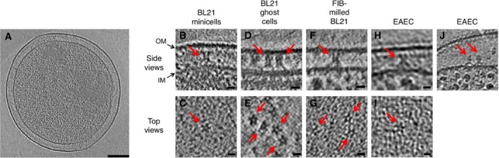
Figure EV1
The TssJLM complex exhibits a C5 symmetry in Escherichia coli BL21 and in EAEC
Slice (13.8u00a0nm) through an engineered BL21 minicell with a diameter of u02dc450u00a0nm. Scale bar 100u00a0nm. Slice (9.7u00a0nm) showing a side view of a TssJLM particle embedded in the cell envel...
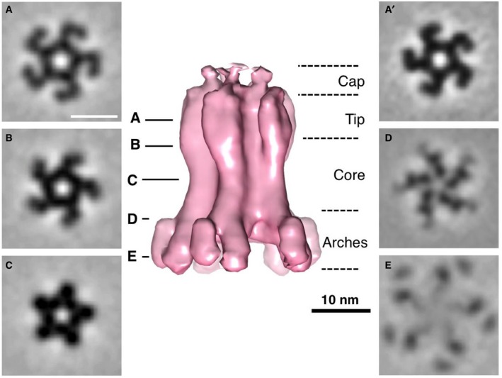
Figure 1
Subtomogram average of the TssJLM complex inu00a0situ
Au2013E Isosurface of the subtomogram average (in pink) with an applied C5 symmetry and 0.69u00a0nm tomographic slices (Au2013E) at the indicated heights. Scale bars 10u00a0nm. The average is shown in...
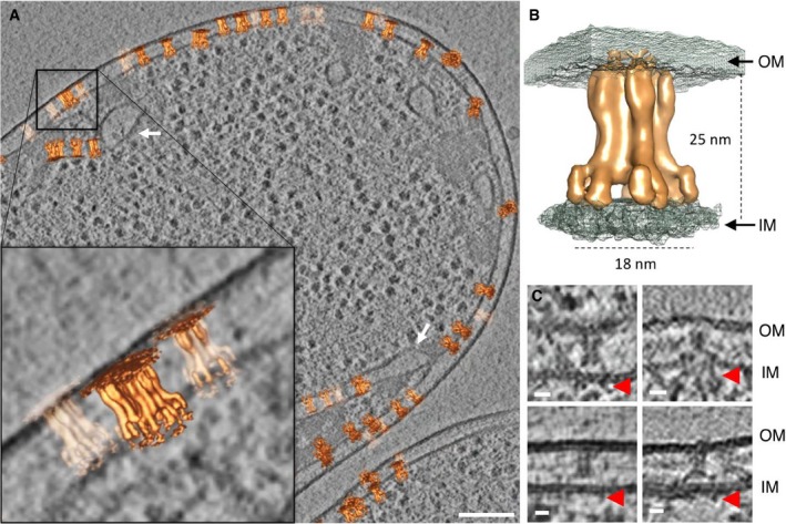
Figure 2
Position of TssJLM in the cell envelope
Slice (9.7u00a0nm) through a cryotomogram of a FIBu2010milled Escherichia coli BL21 cell expressing TssJLM. The average shown in Fig 1 was placed back at the positions and orientations of the individu...
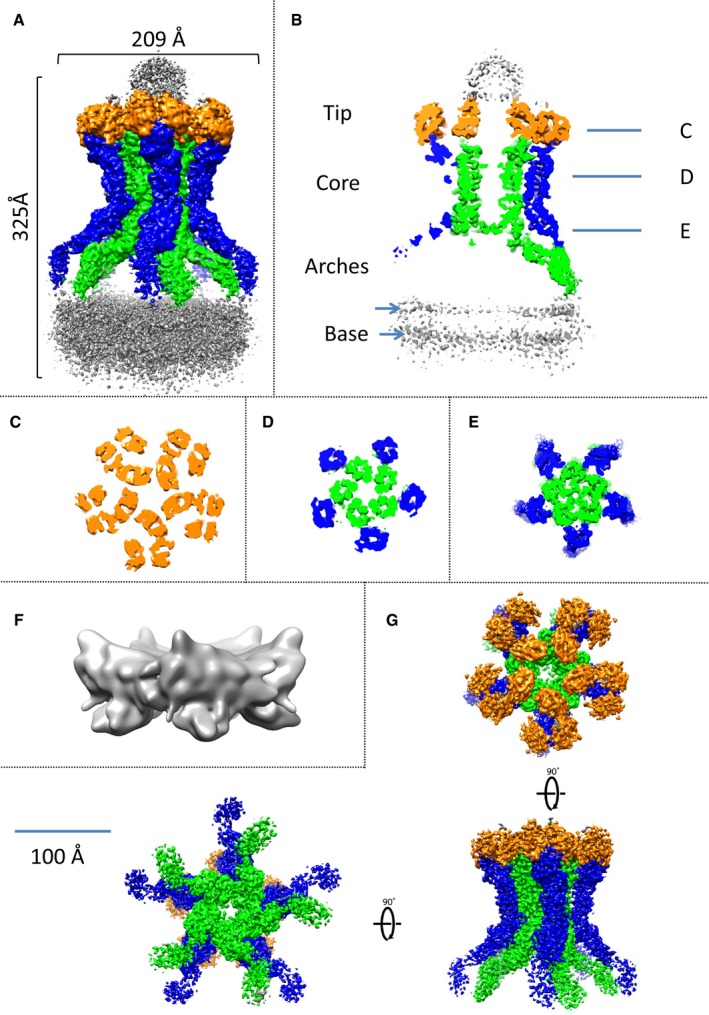
Figure 3
3D structure of the TE complex of the T6SS
A Autosharpened Cryou2010EM density of the full TE complex composed of TssJ, TssL and TssM. The inner pillars are coloured in green and the outer pillars in blue. The unstructured tip and base are in ...
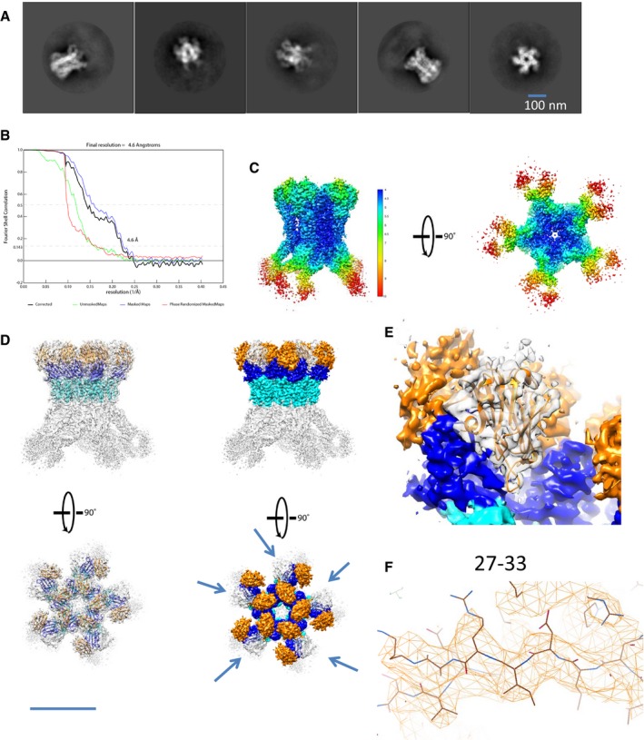
Figure EV2
The cryou2010EM reconstruction of the core of the membrane complex (MC)
2D classes of the subtracted SPA cryou2010EM density corresponding to the core of the MC FSC curve of the core complex as calculated using postu2010process 3D representation of the core 3D reconstruct...
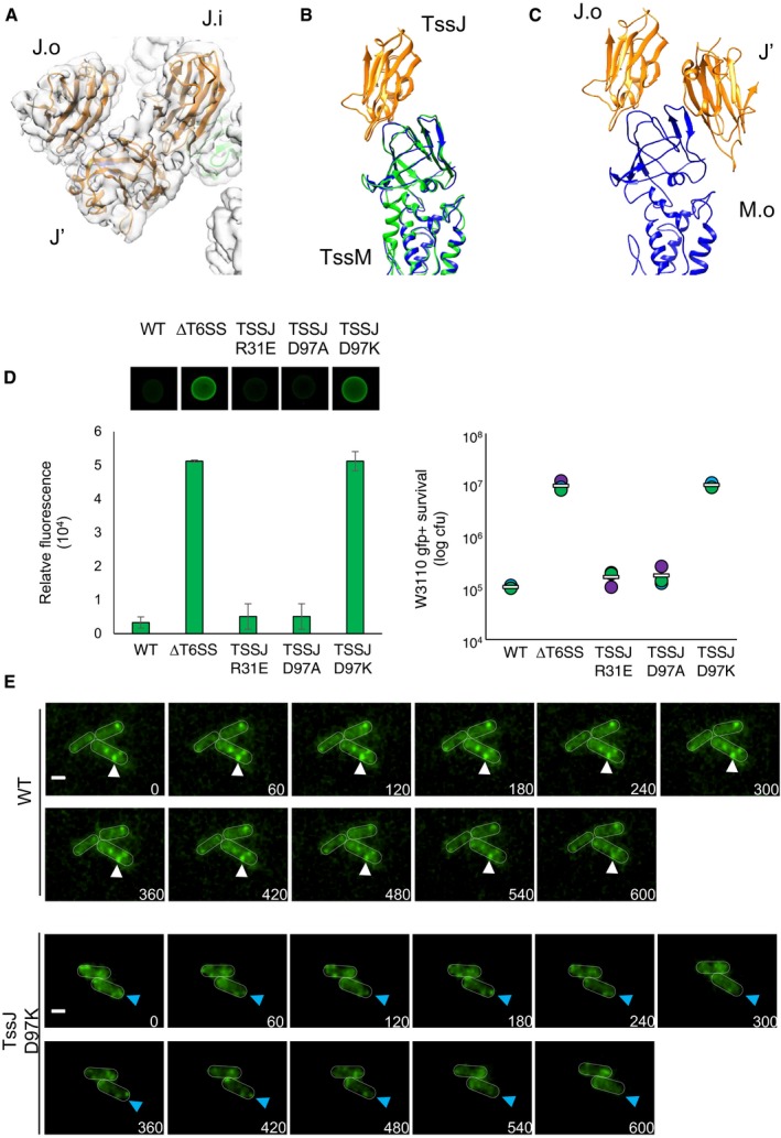
Figure 4
The TssJu2032 monomer and its function
Ribbon diagram and locally sharpened surface representation (transparentu00a0=u00a0of the three TssJ protomers in orange, labelled TssJ.i, TssJ.o and TssJu2032 for the inner, outer and additional mono...
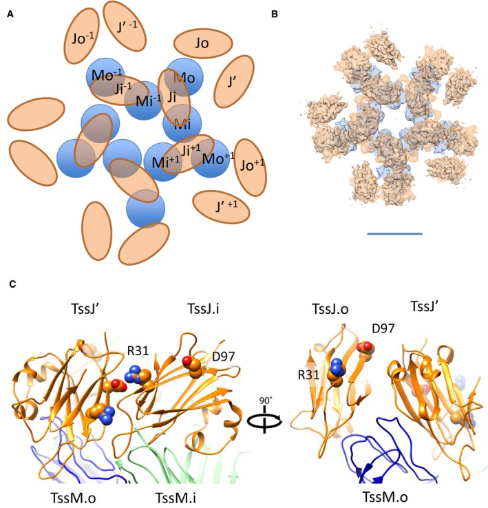
Figure EV3
The TssJu2010TssM assembly
Schematic diagram of the TssMu2010TssJ assembly, labelled according to the nomenclature used throughout this paper. Superimposition of two slices through the MC complex corresponding to TssJ in orange...
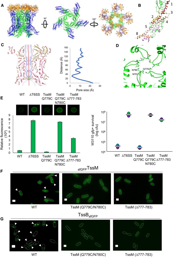
Figure 5
The TssM protein and the periplasmic gate
The highu2010resolution structure of MC complex in different orientations. TssJ is in orange, TssM is in green and blue according to their position as an inner or outer pillar, respectively. Pseudoato...
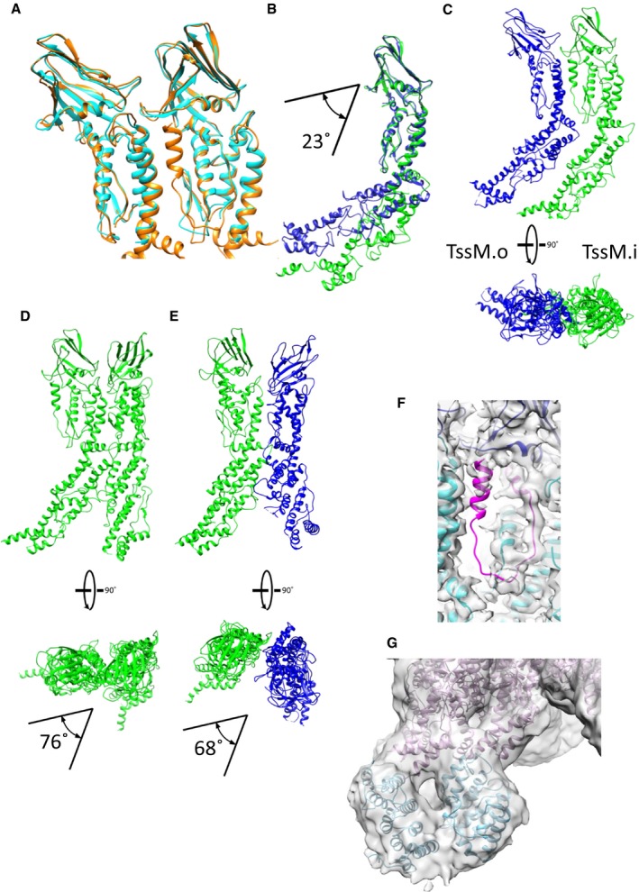
Figure EV4
The TssM pseudoatomic model
Comparison between the TssM from the PDB (4Y7O) in cyan and the refined TssM on the cryou2010EM density in orange. Comparison of the pseudoatomic model of TssM in the internal (green) and in the exter...
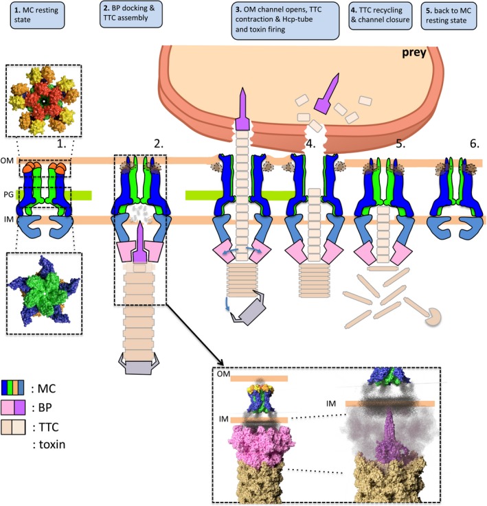
Figure 6
Summary of the Type 6 secretion system cycle of action
The T6SS assembly begins first with the recruitment of the membrane complex (MC) in its resting state (1). The MC recruits the baseplate (BP) and the tail tip complex (TTC) is assembled (2). The recen...
Figure images are served from the NIH/NLM PubMed Central Open Access Subset or Europe PMC; copyright remains with the publishers and authors.
💬 Discussion
0 commentsNo comments yet. Be the first to start a discussion!
Leave a Comment