Abstract
Quantification of cell-cycle state at a single-cell level is essential to understand fundamental three-dimensional (3D) biological processes such as tissue development and cancer. Analysis of 3D in vivo images, however, is very challenging. Today's best practice, manual annotation of select image events, generates arbitrarily sampled data distributions, which are unsuitable for reliable mechanistic inferences. Here, we present an integrated workflow for quantitative in vivo cell-cycle profiling. It combines image analysis and machine learning methods for automated 3D segmentation and cell-cycle state identification of individual cell-nuclei with widely varying morphologies embedded in complex tumor environments. We applied our workflow to quantify cell-cycle effects of three antimitotic cancer drugs over 8 d in HT-1080 fibrosarcoma xenografts in living mice using a data set of 38,000 cells and compared the induced phenotypes. In contrast to results with 2D culture, observed mitotic arrest was relatively low, suggesting involvement of additional mechanisms in their antitumor effect in vivo.
🔬 Techniques
🔭 Microscopes
🧬 Organisms
💻 Software
✨ Fluorophores
🧪 Sample Preparation
🔬 Cell Lines
🏭 Microscope Brands
🧪 Reagent Suppliers
📷 Detectors
🎨 Filters
💻 Software Details
💾 Data Repositories
🏛️ Research Organizations (ROR)
Affiliated research institutions:
📋 Methods
Quantitative analysis of cancer drug effects in space and time
To demonstrate the value of the proposed quantitative imaging workflow, we used it to track the effects of cancer therapeutics on cell cycle progression. This is a particularly difficult problem for an automated imaging pipeline due to the large and unpredictable morphological changes these drugs elicit. We focused on testing effects of cytotoxic cancer drugs that kill cells in mitosis. Most of our current understanding of the mechanism of action of these antimitotic drugs is based on experiments conducted in 2D in vitro cell culture systems that are often inaccurate or incomplete in predicting drug efficacy in patients. While their cytotoxic effects in 2D cell culture are strictly mitosis dependent, increasing evidence suggests that this is likely not the case in human tumors 21 , 22 . To better understand clinical efficacy, we need to measure pharmacodynamics in more realistic environments while maintaining single-cell resolution, as cell cycle arrest and cell death display complex and variable kinetics at the single-cell level 23 . We first analyzed the single-cell pharmacodynamics of the established microtubule (MT)-interacting cancer drug paclitaxel, used in the treatment of breast, ovarian and lung cancer. We followed six tumor positions in a paclitaxel-treated mouse for seven days or as long as the imaging conditions allowed ( Fig. 4a, b, c ). With one exception, the trends in cell density over time were quite similar at all imaged positions ( Fig. 4c ). One position imaged outside the gold grids showed a substantial increase in tumor cell density from day 1 to day 2 after drug treatment, which may be due to the imaging of slightly different locations on different days. This highlights the need for the grid based spatial reference system for accurate tracking of parameters in a defined tumor location. Overall, we measured a downward trend in cell density after treatment with paclitaxel, suggesting that the drug is effective. Cell cycle state quantification showed that mitotic cells accumulated after drug injection, peaking on day 2 ( Fig. 4c ). This was expected for a drug that greatly increases the duration of mitosis by activating the spindle-assembly checkpoint 24 . However, compared to 2D culture models (with up to 80% mitotic cells after 1 day of drug exposure), in our experiments this arrest was much more modest, in line with other in vivo studies 3 , 25 – 27 . To validate the results of the whole imaging and analysis pipeline, we stained tissue sections from paclitaxel treated HT-1080 tumors for the mitotic marker phospho-histone H3 and quantified mitotic arrest by histology as an orthogonal approach ( Fig. 4d , Supplementary Fig. 4 ). The mitotic arrest observed was similar, but slightly lower because the histological approach counts also non-dividing mouse stromal cells while the fluorescent reporters used for intravital microscopy are expressed only in the human graft cells. The proposed intravital imaging pipeline was further validated with flow cytometry of cells from drug treated cancer cell spheroids, an established system for 3D cell culture ( Supplementary Fig. 5 ). Together, these orthogonal validation assays confirmed that application of paclitaxel in vivo induces a relatively low mitotic arrest when compared to 2D culture. To enable more detailed visual inspection of drug effects over time at single-cell resolution, we arranged cell thumbnail images in a montage, grouped by timepoint and predicted cell cycle state ( Fig. 4e ; see Supplementary Fig. 6 for a high resolution version). The distinct color patterns for G1, Late-G1/Early-S and G2 cells allow an immediate, intuitive quantification of the cell cycle distribution: The increase in mitotic cells on days 1 and 2 was accompanied by a concomitant depletion in G1 (red) and early S (yellow cells), probably the result of delayed progression of mitotic cells into the next cell cycle. Beginning with day 3, the trend was reversed. A strong increase in G1/early S cells likely reflects the synchronous transition of the arrested mitotic cells into the next cell cycle. Faulty mitotic exit, called mitotic slippage, is a frequent outcome of prolonged mitotic arrest 28 , 29 . Combined with the metadata and the features calculated for each cell this data presentation approach supports qualitative validation of results and formulation of new hypotheses on the mechanism of drug action in vivo .
Show full methods section
Quantitative analysis of cancer drug effects in space and time
To demonstrate the value of the proposed quantitative imaging workflow, we used it to track the effects of cancer therapeutics on cell cycle progression. This is a particularly difficult problem for an automated imaging pipeline due to the large and unpredictable morphological changes these drugs elicit. We focused on testing effects of cytotoxic cancer drugs that kill cells in mitosis. Most of our current understanding of the mechanism of action of these antimitotic drugs is based on experiments conducted in 2D in vitro cell culture systems that are often inaccurate or incomplete in predicting drug efficacy in patients. While their cytotoxic effects in 2D cell culture are strictly mitosis dependent, increasing evidence suggests that this is likely not the case in human tumors 21 , 22 . To better understand clinical efficacy, we need to measure pharmacodynamics in more realistic environments while maintaining single-cell resolution, as cell cycle arrest and cell death display complex and variable kinetics at the single-cell level 23 . We first analyzed the single-cell pharmacodynamics of the established microtubule (MT)-interacting cancer drug paclitaxel, used in the treatment of breast, ovarian and lung cancer. We followed six tumor positions in a paclitaxel-treated mouse for seven days or as long as the imaging conditions allowed ( Fig. 4a, b, c ). With one exception, the trends in cell density over time were quite similar at all imaged positions ( Fig. 4c ). One position imaged outside the gold grids showed a substantial increase in tumor cell density from day 1 to day 2 after drug treatment, which may be due to the imaging of slightly different locations on different days. This highlights the need for the grid based spatial reference system for accurate tracking of parameters in a defined tumor location. Overall, we measured a downward trend in cell density after treatment with paclitaxel, suggesting that the drug is effective. Cell cycle state quantification showed that mitotic cells accumulated after drug injection, peaking on day 2 ( Fig. 4c ). This was expected for a drug that greatly increases the duration of mitosis by activating the spindle-assembly checkpoint 24 . However, compared to 2D culture models (with up to 80% mitotic cells after 1 day of drug exposure), in our experiments this arrest was much more modest, in line with other in vivo studies 3 , 25 – 27 . To validate the results of the whole imaging and analysis pipeline, we stained tissue sections from paclitaxel treated HT-1080 tumors for the mitotic marker phospho-histone H3 and quantified mitotic arrest by histology as an orthogonal approach ( Fig. 4d , Supplementary Fig. 4 ). The mitotic arrest observed was similar, but slightly lower because the histological approach counts also non-dividing mouse stromal cells while the fluorescent reporters used for intravital microscopy are expressed only in the human graft cells. The proposed intravital imaging pipeline was further validated with flow cytometry of cells from drug treated cancer cell spheroids, an established system for 3D cell culture ( Supplementary Fig. 5 ). Together, these orthogonal validation assays confirmed that application of paclitaxel in vivo induces a relatively low mitotic arrest when compared to 2D culture. To enable more detailed visual inspection of drug effects over time at single-cell resolution, we arranged cell thumbnail images in a montage, grouped by timepoint and predicted cell cycle state ( Fig. 4e ; see Supplementary Fig. 6 for a high resolution version). The distinct color patterns for G1, Late-G1/Early-S and G2 cells allow an immediate, intuitive quantification of the cell cycle distribution: The increase in mitotic cells on days 1 and 2 was accompanied by a concomitant depletion in G1 (red) and early S (yellow cells), probably the result of delayed progression of mitotic cells into the next cell cycle. Beginning with day 3, the trend was reversed. A strong increase in G1/early S cells likely reflects the synchronous transition of the arrested mitotic cells into the next cell cycle. Faulty mitotic exit, called mitotic slippage, is a frequent outcome of prolonged mitotic arrest 28 , 29 . Combined with the metadata and the features calculated for each cell this data presentation approach supports qualitative validation of results and formulation of new hypotheses on the mechanism of drug action in vivo .
Online Methods
Generation of cell line with stable reporter expression and cell culture The HT-1080 cell line (ATCC) was grown in Eagle’s Minimum Essential Medium (EMEM, ATCC 30-2003) supplemented with 10% FBS (Gibco) and 100 units/mL penicillin and 100 μg/mL streptomycin (Gibco) at 37°C with 5% CO 2 . The FUCCI system allows discrimination between G1 and S/G2/M phases of the cell cycle in living cells using a fragment of the G1 specific protein hCdt1 labeled with a red fluorescent protein (mKO2 - hCdt1) and a fragment of geminin labeled with a green fluorescent protein (mAG - hGem), expressed during S, G2 and M phases of the cell cycle 6 . The H2B CFP signal can be used to detect chromosome condensation during mitosis 3 and thus distinguishes interphase from mitosis. To generate a HT-1080 population stably expressing the FUCCI reporter proteins and H2B CFP, the cell line was serially transduced with lentiviral particles coding for mKO2-hCdt1 (neomycin resistance gene), mAG-hGeminin (blasticidin resistance gene) and H2B CFP (hygromycin resistance gene), respectively and kept under continuous selection using the corresponding antibiotics for at least three weeks (1 mg/ml neomycin, 10 μg/ml blasticidin, and 100 μg/ml hygromycin). Fugene6 (Roche) was used for transfection of plasmids into HEK293T packaging cells according to the manufacturer’s protocol. After transfection of viral production plasmids, medium was replaced after 12 hours, and viral supernatant harvested 24 hours later. Cells were transduced and expression of the fluorescent reporter was verified by fluorescence microscopy. A stable, clonal population of cells expressing all three reporter proteins as brightly as possible and with uniform intensity was obtained by limiting dilution to isolate single cell clones on a 96 well plate under antibiotic selection. MCF7 and T47D cell lines were obtained from ATCC and grown in RPMI 1640 (Gibco) supplemented with 10% FBS (Gibco) and 100 units/mL penicillin and 100 μg/mL streptomycin (Gibco) at 37°C with 5% CO 2 . Stable H2B GFP expressing cell lines were generated by K. Krukenberg (Harvard Medical School, Boston, MA) following standard protocols. All cell lines were obtained as mycoplasma free aliquots from ATCC and not tested in house for mycoplasma contamination.
Mice
All procedures and animal protocols were approved by the subcommittee on Research Animal care at Massachusetts General Hospital. Nu/Nu mice (Cox-7; Massachusetts General Hospital) were fed 5 ml antibiotic (sulfamethoxazole/trimethoprim 200 mg/40 mg per 5 ml; Aurobindo Pharma) in 250 ml drinking water with weekly changes during the length of the experiment. For dorsal skinfold chamber (DSC) implantation, cell injection, injection of drugs, and microscopy, mice were anesthetized by isoflurane vaporization (Harvard Apparatus) with 2.0 L/min isoflurane: 2.0 l/min oxygen. After 30 min of imaging, the isoflurane flow rate was slowly reduced to less than 1.5 l/min. One hundred microliters of saline was injected i.p. every hour during imaging to maintain hydration. Surgery was conducted under sterile conditions with a zoom stereomicroscope (Olympus SZ61). To reduce discomfort mice were treated with analgesic (buprenorphine 0.1 mg/kg, Patterson Veterinary Supply) prior to surgery and every 12 hours for three days after surgery. DSC implantation Titanium DSCs (APJ Trading Co, Inc.) were implanted into the dorsal skinfold of Nu/Nu mice as described 3 The DSC stretches and sandwiches the 2 layers of skin on the back of the mouse. On one side, the skin is surgically removed and replaced by a 10-mm-diameter optical glass cover slip held in place with a c-clip. Spacers between the two halves of the DSC frame prevent excess compression of the tissue and vessels. The window allows free-access imaging of the remaining layers of striated skin muscle, subcutaneous tissue, deep dermis, and tumors.
Cell injection into DSC
Cells were harvested by trypsinization (0.25% trypsin-EDTA) and resuspended in growth medium. Preliminary studies with this three-color cell line grown in xenograft tumors showed a mean segmentation accuracy in the crowded tumor environment of 83.84% ( Supplementary Fig. 1 ). We therefore reduced fluorescent cell density by mixing fluorescent cells 1:20 or 1:35 with the non-fluorescent parental cell line. These ratios were chosen as an empirical optimum between segmentability and having enough cells per image to collect reliable statistics ( Supplementary Fig. 2 ), and resulted in an actual proportion of 20–80% of labeled tumor cells after engraftment. After DSC implantation and cell injection, tumors were allowed to vascularize and grow for 2–3 weeks with the non-fluorescent parental cell line. Mice were anesthetized and approximately 2×10 6 (50 μl) cells were injected subcutaneously into the DSC using a 0.5 ml insulin syringe (29G; BD Biosciences). The needle was bent at 90 degrees to aid injection. Injections were carried out under a stereomicroscope. After injection, sterile saline was added into the DSC and it was closed with a new cover slip. Before imaging, DSCs and tumors were evaluated and rejected if there were any gross tissue abnormalities, the possibility of tissue movement, necrosis or infection.
Grid implantation
To allow reliable identification of the same tumor region during consecutive imaging sessions we tested different techniques such as the use of fluorescent fiducial beads, vascular landmarks, relative position to the external metal frame of the DSC and the use of various metallic grids. Gold grids with mesh size of 75G routinely used in electron microscopy proved most reliable for imaging the same regions repeatedly. One day before the first imaging session the cover slip was removed, and a 75 mesh gold grid (G-75-G; Energy Beam Science, CT, USA) was carefully positioned onto the tumor, covered with saline, and the DSC closed with a fresh cover slip. The grid attaches to the tumor and tumor cells grow between and over the gold grid. As a result the tumor moves with the grid if it shifts in small increments. The grid size was selected so that the imaging field (25x objective with 2 zoom) is just inside of the grid openings and does not include the gold frame.
Drug treatment
Random animals were assigned to each treatment group. To allow neovascularization, HT-1080 xenografts were grown for 2 to 3 weeks before drug treatment. For our experiments, we selected a single dose between 50–70% of published maximally tolerated doses. Mice treated with paclitaxel were injected in the tail vein with a single bolus of 30 mg/kg paclitaxel (injectable formulation, Novaplus; Bedford Laboratories). A total of 30 mg/kg paclitaxel was used based on published data 26 , 35 . Eribulin (Halaven) was injected in the injectable formulation (Eisai) into the tail vein at a dose of 1.2 mg/kg 31 . The KSP inhibitor SB-715992 (ispinesib, Seleckchem) was dissolved in 10% Ethanol, 10% Cremophor EL (Sigma Aldrich) and 80% D5W (5% w/v aqueous dextrose solution) according to published protocols 30 and injected intraperitoneally. The dose of 20 mg/kg body weight was selected based on the data in AACR 2002, Poster 1335, available from http://www.cytokinetics.com/pdf/AACR_2002_Poster_1335.pdf , where the MTD in female BDF mice was determined as 36 mg/kg.
Microscopy
To reduce motion artifacts and permit high-resolution microscopy over extended periods, a custom made DSC holder was used 3 The setup consists of an aluminum holder attached to an aluminum platform. The platform and DSC holder were kept at 38°C to reduce thermal drift. The screws of the DSC fit into machined holes in the holder and the DSC frame was further immobilized using small plates and screws. The microscope was mounted on a floating air table to eliminate vibration external to the instrumentation. A customized Olympus FV1000 confocal/multi-photon microsocope was used. Olympus objectives were as follows: 25× XPlan N [numerical aperture (NA) = 1.05, water], 2×/340 XLFluor (NA = 0.14, air). Because of the significant advantages of 2 photon excitation in depth penetration and tissue we tried to excite all 3 channels using 2 photon excitation. However, with the lasers currently available in our laboratories, it was not possible to efficiently excite mKO2 and achieve clean channel separation with 2 photon imaging. Thus, to achieve the best image quality possible for nuclear segmentation, the H2B channel was acquired using two-photon microscopy while the red and green FUCCI channels were re-acquired in a second run using single-photon laser-scanning confocal microscopy. Monomeric Azami Green (mAG) and monomeric Kusabira Orange (mKO2) were excited using a 473 nm or 559 nm pumped diode laser, respectively, in combination with a DM405/473/559-nm dichroic beam splitter. Emitted light was separated and collected with beam splitters SDM560 and SDM640 and band-pass filters BA490-540 and BA575-620. In addition, each z-stack was acquired using two-photon excitation at 830 nM with a FV10-MRCYR/XR filter cube (Olympus) to image H2B CFP. Using a motorized xy stage, three to ten z-stacks of 20 to 50 optical sections (2 μm per section), were collected. With these acquisition conditions, in some cases, the faster attenuation of green fluorescence intensity with depth vs. red may cause some yellow (Late-G1/early S) cells to appear red. If this issue is relevant to the question addressed, our computational framework offers cell cycle models where red and yellow cells are pooled to avoid this possible issue. The grid based tracking method used here is only suitable for treated tumors or tissues with low proliferation rates. If untreated, proliferating tumor cells tend to overgrow the grid within a few days. Image quality during intravital imaging can be affected by many factors, like edema formation, growth of fibrous tissue over the tumor, tissue drift (i.e. drift of the tumor tissue away from the cover slip), all of which can also be induced by drug treatment. When assessing the growth or recession of tumorous tissue, it is important to ensure that changes in cell count are not due to such phenomena. This can be reliably judged by the appearance of the images: very weak contrast or, in general, uniform reduction in the signal to noise ratio reflects one of the problems mentioned above. When individual positions showed such problems at late timepoints, tracking was stopped. In general, rarely encountered problems with image quality up to day 7 post-treatment, but later timepoints showed major variation, and we would not recommend experiments longer than 8 days. In other xenograft systems or when unperturbed tissues are imaged, longer imaging may be possible. Histopathological analysis Unlabeled HT-1080 tumors were either left untreated or treated with a single dose of 40 mg/kg paclitaxel i.v. for 1, 4 or 7 days. Three tumors for each condition were embedded in O.C.T. compound (Sakura Finetek) and serial 6 μm-thick frozen sections were prepared for histopathological analysis. For immunohistochemistry, the tissue sections were treated with 0.3% H 2 O 2 in dH 2 O to suppress endogenous peroxidase activity, and then blocked using 4% goat normal serum in PBS for 30 minutes at room temperature. The sections were incubated with a primary antibody, phospho-histone H3 (Ser10) (1:200, #9710, Cell Signaling), overnight at 4°C. The following day, the sections were washed in PBS three times for five minutes each and incubated with biotinylated anti-rabbit IgG (1:100, BA1000, Vector Laboratories) for 30 minutes at room temperature. After washing the sections in PBS three times for 5 minutes each, VECTASTAIN ABC kit (Vector Laboratories) was applied according to the manufacturer’s protocol, and a 3-amino-9-ethylcarbazole (AEC) substrate (Dako) was used for color development. All the sections were counterstained with Harris hematoxylin (Sigma-Aldrich) and images were captured using NanoZoomer 2.0RS (Hamamatsu).
Spheroid culture experiments and imaging
Cancer cell line spheroids were grown as described 36 . Briefly, 10000 cells per well were seeded in 96 well plates (Greiner Bio-One, 655090) coated with 1.5% agarose dissolved in complete growth media and polymerized at room temperature. Half the media was exchanged every 2–3 days. Three to six days after plating, spheroids were moved for imaging to 96 well plates coated with Poly-HEMA as described 37 . At this point, the spheroids had usually reached a diameter >300μM. Imaging was performed on a Nikon Ti motorized inverted microscope equipped with a Yokagawa CSU-X1 spinning disk confocal head with Spectral Applied Research Aurora Borealis modification and Spectral Applied Research LMM-5 laser merge module with AOTF controlled solid state lasers. A 445nm (80mW) laser was used to excite CFP, a 488nm (100mW) laser for mAG and GFP and a 561nm (100mW) laser to for mKO2. Images were acquired with a Hamamatsu ORCA-AG cooled CCD camera controlled by MetaMorph image acquisition software in whole media at room temperature. The following lasers and filter sets were used: CFP: Excitation: 447nm, Dichroic: Triple 447/515/642, Emission: 480/40; mAG/GFP: Excitation: 491nm, Dichroic: QUAD 405/491/561/642, Emission: 525/50; mKO2: Excitation: 561nm, Dichroic: QUAD 405/491/561/642, Emission: 620/60. The typical depth of z-stacks was 40–50μM, binning was set to 1 and the z spacing was 2μm.
Flow cytometry of spheroids
In the flow cytometry validation experiments ( Supplementary Fig. 5 ), 96 HT-1080 spheroids were grown per treatment condition on 96 well Nunclon Sphera U-Bottom plates with a nonadherent surface (Thermo Scientific, 174925) for 4 days. Then, three spheroids per condition were treated with either 2 μM paclitaxel or DMSO as a control for 18 hr and imaged on poly-HEMA coated plates as described above. Immediately after imaging, all 96 spheroids were pooled for each condition and spun down by centrifugation (400g for 5 min), followed by dispersion of the pellet into a single-cell suspension in 100 μl 0.25% Trypsin solution. After 1 min of trypsin treatment, cells were resuspended by pipetting, 1ml of complete culture media was added and 500μl of the suspension were transferred into FACS tubes. Living cells were stained with DyeCycle Violet dye (Molecular Probes, V35003) at a concentration of 10 μM for 20 min at 37°C and analzyed on a BD LSRII flow cytometer. The dye was excited with a 405 nm laser and emitted fluorescence was detected with a 450/50 bandpass filter. For data analysis, FlowJo v.X.0.7 was used. First, living single-cells were gated through a FSC/SSC live cell gate combined with a single-cell gate on the Alexa Fluor 405-A vs. Alexa Fluor 405-W plot. This population was then analyzed using the built in cell cycle quantification platform using the univariate model without any adjustments.
Nuclei segmentation
Firstly, the images were preprocessed by applying a 3×3×3 median filter to reduce noise. Then, a rough foreground-background segmentation was obtained using a Poisson-based minimum error thresholding method 38 , wherein the image histogram is modeled as a mixture of two poisson models, one for the foreground and one for the background, and the threshold is computed by minimizing the relative entropy between the image histogram and the poisson mixture model. Because of the high variability in foreground-background contrast, caused by attenuation of intensity values with depth and by changes in the brightness of cell nuclei depending on their cell cycle state, applying a global threshold to the entire 3D volume did not provide an accurate segmentation. To address this issue, the thresholding method was applied in a locally adaptive fashion within each slice of the 3D volume. The result obtained was then cleansed with a set of refinement steps that included hole-filling, morphological opening to remove thin structures such as vessels and the removal of small regions such as fragments of dead cells whose size is below a sanity threshold. Typically, the choice of a good thresholding algorithm varies based on the nature of the data being analyzed and the aforementioned approach may not yield an optimal performance on other biological systems and/or data acquired using other microscopic setups. Hence, our software provides a set of foreground-background segmentation algorithms, each of which was found to work better in specific scenarios, that the user can quickly try on sample data and pick a method that works well. Next, seed points were detected in the cell nuclei by analyzing the response of a scale-adaptive multiscale Laplacian-of-Gaussian (LoG) filter. Specifically, the filter was applied at a series of scales within a user-specified scale-range and the local maxima in the 4D scale-space response were defined as seed points. This multiscale approach provides scale-invariance enabling the detection of seed points in nuclei with varying size. While searching for local maxima, the use of a constant scale-range for all voxels led to inaccurate results, especially for clusters of nuclei of different sizes touching each other with weak edge information in between. Al-Kofafi et. al. proposed an elegant solution 17 to this problem in the context of nuclei segmentation in 2D histopathological images. The authors incorporated a finer per-pixel control over the scale-range using the Euclidean distance map of the binary foreground-background mask. Specifically, they constrained the upper-bound of the scale-range to that of a blob with radius equal to the distance map value at each voxel. Here, we adapt this method to the context of nuclei seed point detection in 3D intravital images. The detected seed points were then used as markers for the marker-controlled watershed algorithm 18 , 19 on the negative response of the multi-scale LoG filter to obtain an initial segmentation result. (Background regions were pruned by computing an intersection with the foreground mask obtained using the thresholding method). This result, however, was unsatisfactory, especially in cases where nuclei of different sizes and/or shapes touch each other and when nuclear shape is aspherical. Both scenarios often occur in our data and became increasingly profound drug treatment. This leads to the detection of multiple seed points within a single nucleus resulting in over-segmentation errors or to the detection of a single seed point for a cluster of touching nuclei resulting in under-segmentation errors. The relative proportion of these two types of errors can be manipulated by tuning the scale-range parameter of the multi-scale LoG filter. Decreasing the lower-bound of the scale-range results in relatively more over-segmentation errors and increasing it results in relatively more under-segmentation errors. Since it is hard to design a principled approach to correct under-segmentation errors, we chose to intentionally over-segment the nuclei by pushing down the lower-bound of the scale-range to a value that empirically results in little or no under-segmentation errors and then correct the over-segmentation errors using a region merging approach. There have been a few interesting efforts reported in the literature that adopt a similar but varied strategy to correct over- and under-segmentation errors resulting from the use of the watershed algorithm for 3D cell nuclei segmentation 12 – 16 and the method proposed here is based on constructive insights drawn from each of them. The most promising of these is a series of three incremental and increasingly effective methods proposed by Lin et.al. 13 , 15 , 16 wherein adjacent regions in the result obtained from the watershed algorithm are iteratively merged in a greedy fashion based on confidence scores derived from a generative classification model. The key ingredient of success in their method is the underlying generative model, which constitutes a probabilistic model of a well-segmented cell nucleus based on a set of features quantifying the appearance, boundary edgeness, size, and shape of the region. However, given the high amount of heterogeneity in the size, shape and appearance of the cell nuclei in our data exacerbated further by the action of cancer drugs, it becomes difficult to design an accurate probabilistic model that encompasses all of the nuclei irrespective of whether a parametric or a non-parametric distribution is employed. On the contrary, for the present task of region merging, one has to only decide whether or not to merge a given pair of mutually adjacent regions. This is relatively less complicated than answering the more general question of whether or not a given region is a well-segmented cell nucleus. These insights suggest that the use of a purely discriminative classification approach may be more amicable to adopt than a generative one which is also in line with the widely believed design philosophy articulated succinctly by Vapnik 39 that “one should solve a problem directly and never solve a more general problem as an intermediate step”. For a very similar line of reasoning discriminative classifiers in general are known to perform better than their generative counterparts 40 . Based on these inferences, we chose to guide the region merging process using a discriminative classification model with a richer set of image-derived features carefully designed to just solve the classification problem at hand. Given an initial segmentation of the cell nuclei obtained from the marker-controlled watershed algorithm, a supervised hierarchical learning-based region merging approach was used to detect and correct any over-segmentation errors. Firstly, a non-negative edge-weighted region adjacency graph (RAG) was constructed wherein each vertex represents a distinct region in the watershed segmentation result and the edges connect vertices corresponding to the regions that share a common boundary in the image space. The weight of an edge connecting two vertices represents the confidence in merging the associated regions to correct a potential over-segmentation error computed using a two-class classification model that is trained to detect over-segmentation errors. Specifically, if the classifier senses a potential over-segmentation error and recommends merging of two adjacent regions, then the corresponding edge-weight in the RAG is set equal to the classifier’s prediction probability for the merge decision. If the classifier recommends against merging a given pair of adjacent regions, then the corresponding edge is removed from the RAG. After graph construction, adjacent regions were iteratively merged in decreasing order of merge confidence given by the weight of the corresponding edge in the RAG. In each iteration of the region merging process, the edge with maximum weight in the RAG was picked, the two associated regions were merged and the RAG was updated by recomputing the weights of the edges to all the neighboring regions using the classification model thereby allowing the regions to be merged in a hierarchical fashion. To efficiently carry out the operations of retrieving the edge with maximum weight in each iteration and subsequently updating the RAG, all the edges of the RAG were added to a heap-based max-priority queue data structure with edge-weights as priorities. Additionally, before adding an edge to the priority queue, a check was performed to make sure it has a dominant weight among its neighboring edges to instill an extra amount of confidence into the merge-decision 41 . The key component of success in the proposed region merging method is the underlying discriminative two-class classification model that decides whether or not to merge two adjacent regions using a carefully designed set of image-derived features. The classification model was built in a supervised fashion from a semi-automatically generated training set containing examples of both merge and don’t-merge classes: (i) the merge class contains pairs of adjacent regions that belong to a single-cell nucleus that was over-segmented by the watershed algorithm, and (ii) the don’t-merge class contains pairs of adjacent regions that belong to two distinct cell nuclei. To efficiently obtain the necessary training data, deliberately over-segmented results were generated using the watershed algorithm and presented to a human expert in the form of a user-friendly software tool. The tool allowed manual classification of each segmented region/fragment as over-segmented, under-segmented, or well-segmented. Isolated pairs of adjacent over-segmented regions with no other regions beside them were then extracted and used as examples of the merge-class. Pairs of adjacent regions in which either both or one was correctly segmented were extracted and used as examples of the don’t-merge class. The generated training dataset was then used to train a two-class random forest classifier 42 to decide whether a given pair of adjacent regions should be merged or not based on a set of 20 image-derived features categorized in three groups, namely: (i) appearance similarity group containing features quantifying the similarity in appearance of the two adjacent regions in terms of overall brightness, intensity distribution, and texture, (ii) boundary saliency group containing features quantifying the amount of edge information at the common boundary shared by the two regions which we refer to as the watershed region, (iii) boundary continuity group containing features quantifying the continuity in the bounding surfaces of the two regions in terms of curvature at the neck, the amount of shared boundary, the gap between the bounding surfaces of the two regions, and the change in convexity introduced by a potential region merging decision ( Supplementary Table 1 , Fig. 2b ). Additionally, to prevent the heavy imbalance between the proportions of examples in the merge and don’t-merge classes in our training dataset from biasing the classifier towards the majority class, an ensemble of five random forest classifiers was created wherein each component of the ensemble is trained on a randomly under-sampled balanced subset of the training data. In the test phase, the final classification decision was made by fusing the decisions of all the components in the ensemble using the average of probabilities rule. Lastly, after the region merging process, segmented regions touching the image border in the X and Y dimensions and whose size and volume are below a sanity threshold were pruned. Note, that only the nuclear marker channel was used to segment cell nuclei for two primary reasons: (i) all the nuclei are visible in the nuclear marker channel at all time points, unlike the FUCCI cell cycle marker, and (ii) future studies may rely on other biosensors to study different aspects of chemotherapeutic drug action. Automatic cell cycle state identification Firstly, the two FUCCI channels were aligned to the histone channel using a masked image registration algorithm. This was necessary because the FUCCI and histone channels were acquired in single- and two-photon fluorescence imaging modalities, respectively. A purely translational transform was sufficient in our case, however, the following procedures would also be applicable to more complex misalignments such as rotation. Since only a subset of cell nuclei present is visible in the FUCCI channels, it would be inaccurate to use all the voxels in the volume to compute the similarity metric in the registration algorithm. To address this problem, a rough estimate of the foreground in each of the two FUCCI channels was obtained using the Otsu thresholding algorithm 43 and then only the voxels inside the estimated foreground mask were used to compute the similarity metric in the registration algorithm. The registration was done in a multi-scale fashion using the Elastix registration toolkit 44 with an adaptive stochastic gradient descent optimizer and the mutual information metric. After aligning the channels, each detected cell was represented by 73 quantitative features computed from the histone and/or FUCCI channels ( Supplementary Table 4 ) encoding two different but complementary characteristics: (i) histone feature group containing features characterizing the appearance of the cell nucleus in the histone channel using a set of intensity statistics, Haralick texture features 45 computed at multiple scales, and a few geometric features quantifying the shape of the cell nucleus, and (ii) the FUCCI feature group containing features characterizing the appearance of the cell nucleus in the FUCCI channels using a set of intensity statistics computed from each of the two FUCCI channels and a set of measures quantifying the relative dominance and colocalization between channels using the Pearson correlation coefficient and the ratios of a selected set of intensity statistics between channels. The features in the FUCCI group are effective in distinguishing cells in G1, Late-G1/Early S, and S/G2/mitosis, and the features in the histone group are effective in distinguishing a cell in mitosis from others ( Fig. 3c ). A random forest classifier 42 was trained with a database of manually labeled cell nuclei ( Fig. 3b ) to automatically identify the cell cycle state of each cell given its representation in the high-dimensional feature space. To prevent the heavy class imbalance in the training dataset from biasing the classification, an ensemble of five random forest classifiers was created wherein each component of the ensemble is trained on a randomly under-sampled balanced subset of the training data. In the test phase, the final classification decision was made by fusing the decisions of all the components in the ensemble using the average of probabilities rule. The aforementioned classification scheme was then applied to build a four-class model that associates a given cell to: (i) G1, (ii) Late-G1/Early S, (iii) S/G2, or (iv) mitosis. Additionally, to facilitate studies that want to monitor the cell cycle progression at a coarser level, the same classification scheme was used to build two dedicated and more accurate two-class models: (i) Interphase vs mitotic model to distinguish cells in Interphase (G1 + Late-G1/Early-S + S/G2) against mitotic cells, and (ii) G1 vs S/G2/mitotic model to distinguish cells in G1 phase from the cells in S, G2, and mitotic phases of the cell cycle.
Software
The proposed computation framework was mostly implemented in MATLAB (Mathworks) taking advantage of its parallel computing toolbox to reduce computational time when multiple processing cores are available. We used a machine learning library called WEKA 46 to explore, design, conceptualize, train, and validate all the machine learning models used in our framework and we interface our software with Imaris (Bitplane) for 3D visualizations. Manual annotation of all training datasets was performed blinded. The plots in the paper were generated using MATLAB, Python and Mathematica 9 (Wolfram Research) and plotly (www.plot.ly). Total computational time, including both nuclei segmentation and cell cycle state identification, for a typical volume of size 512×512×40 voxels with 200–600 cells is 5–10 minutes on a desktop workstation with 8 processing cores (2.93 GHz per core) with 12 GB of RAM and 10–20 minutes when run on a single processing core. The software and the underlying source code will be made publicly available for use by the scientific community as a supplementary file and under http://lccb.hms.harvard.edu/doc/InvivoCytometer_v2.0.zip . It includes a user-friendly interface for biologists and is implemented in a modular way so the nuclear segmentation algorithm can be used to address biological questions requiring other reporter systems. Statistical analysis In Fig. 5 , we used Dunnett’s t-test to compare the mean values (normalized cell density, percentage of cells in each cell cycle state) computed accross different positions within the tumor on each day after drug treatment with the pre-drug time point, and a one-sided regression slope t-test to check if there is a significant downward trend in the cell density over time. In Fig. 6 , we used the one-sided t-test to see if there is a significant increase in multinucleation 3-days after drug treatment when compared to the pre-drug time point. For both figures, since the variation seen at each timepoint is across different locations in the same tumor the test statistic was assumed to be normally distributed. All statistical tests were performed using JMP Pro 11.0.0 (SAS).
Supplementary Material 1 2
📊 Figures
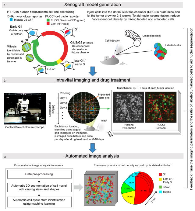
Figure 1
Overview of experimental setup and image analysis Panel 1
Generation of xenograft tumors. HT-1080 cells engineered to stably express the FUCCI cell cycle reporter system and Histone H2B CFP allow in vivo detection of G1, Late-G1/Early-S, S/G2 and mitotic cel...
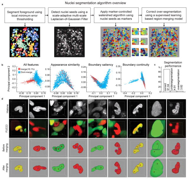
Figure 2
Automatic segmentation of cell nuclei
(a) Steps of segmentation algorithm. Intermediate results of each step are visualized in 3D. Parameters of the seed point detection filter are tuned to lean towards over-segmentation of the nuclei whi...
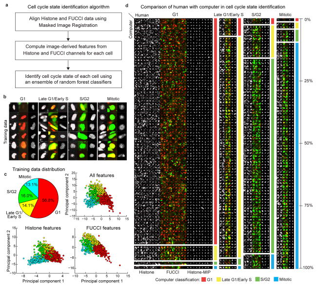
Figure 3
Automatic identification of cell cycle state
(a) Steps of cell cycle state identification algorithm. (b) Examples of cells from each cell cycle state in our training dataset. (c) Class distribution (top-left) in training dataset and 2D projectio...
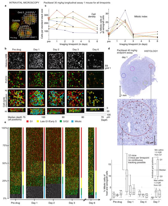
Figure 4
Quantitative analysis of drug response to paclitaxel treatment at a single-cell level
Analysis of an HT-1080 tumor treated with a single dose (30 mg/kg) of the MT-interacting drug paclitaxel and validation by histology. (a) Two gold grids allow tracking of tumor positions over time, be...
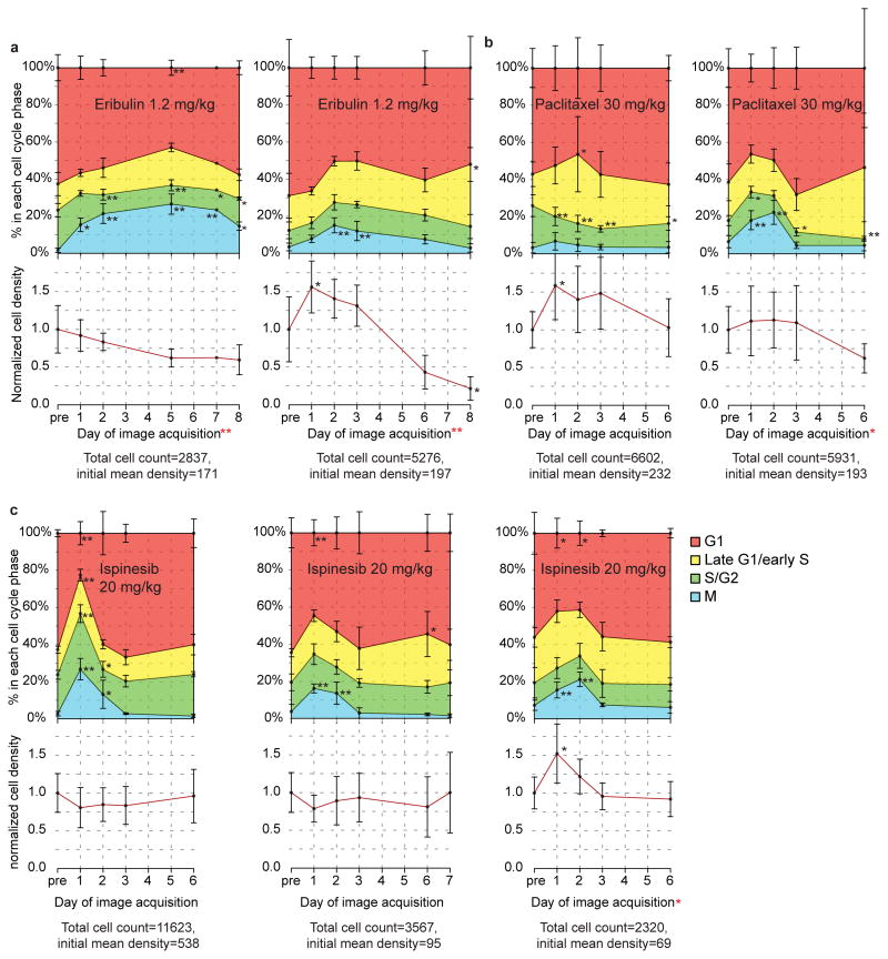
Figure 5
Pharmacodynamics of antimitotic drugs in the HT-1080 xenograft system
Effects of three different antimitotic cancer drugs compared as in Fig. 4 . Each plot shows data from one mouse. Upper half: cell cycle state distribution. Lower half: mean cell density over time. (a)...
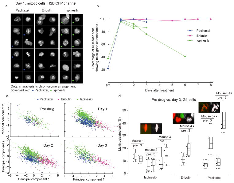
Figure 6
Antimitotic drugs induce different mitotic and interphase phenotypes
Examples of cell morphology induced by antimitotic drugs (same datasets as Fig. 5 ) (a) Random sample of cells imaged on day 1 after drug injection and identified by the analysis framework as mitotic....
Figure images are served from the NIH/NLM PubMed Central Open Access Subset or Europe PMC; copyright remains with the publishers and authors.
💬 Discussion
0 commentsNo comments yet. Be the first to start a discussion!
Leave a Comment