Abstract
Abstract RNA hybridization‐based spatial transcriptomics provides unparalleled detection sensitivity. However, inaccuracies in segmentation of image volumes into cells cause misassignment of mRNAs which is a major source of errors. Here, we develop JSTA, a computational framework for joint cell segmentation and cell type annotation that utilizes prior knowledge of cell type‐specific gene expression. Simulation results show that leveraging existing cell type taxonomy increases RNA assignment accuracy by more than 45%. Using JSTA, we were able to classify cells in the mouse hippocampus into 133 (sub)types revealing the spatial organization of CA1, CA3, and Sst neuron subtypes. Analysis of within cell subtype spatial differential gene expression of 80 candidate genes identified 63 with statistically significant spatial differential gene expression across 61 (sub)types. Overall, our work demonstrates that known cell type expression patterns can be leveraged to improve the accuracy of RNA hybridization‐based spatial transcriptomics while providing highly granular cell (sub)type information. The large number of newly discovered spatial gene expression patterns substantiates the need for accurate spatial transcriptomic measurements that can provide information beyond cell (sub)type labels.
🔬 Techniques
💻 Software
✨ Fluorophores
🧪 Sample Preparation
🔬 Cell Lines
🏭 Microscope Brands
💻 Software Details
💾 Data Repositories
🏛️ Research Organizations (ROR)
Affiliated research institutions:
📋 Methods
JSTA overview and method
Our computational framework of JSTA is based on improving initial watershed segmentation by incorporating cell (sub)type probabilities for each pixel and iteratively adjusting the assignment of boundary pixels based on those probabilities (Fig 1A ). Figure 1 Overview of JSTA and the spatial transcriptomic data used for performance evaluation Joint cell segmentation and cell type annotation (JSTA) overview. Initially, watershed‐based segmentation is performed and a cell‐level type classifier is trained based on the Neocortical Cell Type Taxonomy (NCTT) data. The deep neural network (DNN) parameterized cell‐level classifier then assigns cell (sub)types (red and blue in this cartoon example). Based on the current assignment of pixels to cell (sub)types, a new DNN is trained to estimate the probabilities that each pixel comes from each of the possible (sub)types given the local RNA density at each pixel. In this example, two pixels that were initially assigned to the “red” cells got higher probability to be of a blue type. Since the neighbor cell is of type “blue”, they were reassigned to that cell during segmentation update. Using the updated segmentation and the cell type classifier cell types are reassigned. The tasks of training, segmentation, and classification are repeated over many iterations until convergence.
Multiplexed error robust fluorescent in situ hybridization
(MERFISH) and DAPI stained nuclei in the mouse hippocampus. Each gene is represented by a different color. For the entire hippocampus (left), only the mRNA spots are shown with a scale bar of 500 μm. On the zoomed‐in section (right), each gene is represented by a different color dot, and the DAPI intensity is displayed in white. The scale bar is 20 μm. To evaluate JSTA, we chose to use the mouse hippocampus for two reasons: (i) The mouse hippocampus has high cell (sub)type diversity as it includes more than 35% of all cell (sub)types defined by the NCTT. (ii) The mouse hippocampus has areas of high and low cell density. These two reasons make the mouse hippocampus a good test case for the hypothesis that external cell (sub)type‐specific expression data could be leveraged to increase the accuracy of spatial transcriptomics, as implemented in our approach. We performed multiplexed error robust fluorescent in situ hybridization (MERFISH) of 163 genes which include 83 selected cell marker genes, which show distinct expression between cell types and are used for cell classification and segmentation and 80 genes previously implicated with biological importance in traumatic brain injury (Fig 1B ). Combining this MERFISH dataset, DAPI stained nuclei, and the NCTT reference dataset using JSTA, we created a segmentation map that assigns all mRNAs to cells while simultaneously classifying all cells into granular (sub)types based on NCTT. In JSTA, we leverage the NCTT information to infer probabilities at the pixel level. However, learning these probabilities from NCTT is challenging for two reasons. (i) NCTT data were acquired with scRNAseq technology that has higher sparsity due to low capture rates and needs to be harmonized. (ii) NCTT data provide expression patterns at the cell level and not the pixel level. We expect the mean expression among all pixels in a cell to be the same as that of the whole cell. Yet, variance and potentially higher distribution moments of the pixel‐level distribution are likely different from those of the cell‐level distribution due to sampling and biological factors such as variability in subcellular localization of mRNA molecules (Eng et al, 2019 ). To address these issues, JSTA learns the pixel‐level cell (sub)type probabilities using two distinct deep neural network (DNN) classifiers, a cell‐level type classifier, and a pixel type classifier. Overall, JSTA learns three distinct layers of information: segmentation map, pixel‐level classifier, and cell‐level classifier. Learning of model parameters is done using a combination of NCTT and the MERFISH data. The cell type classifier is learned directly from NCTT data after harmonization. The other two layers are learned iteratively using expectation maximization (EM) approach (Chen et al , 2015 ). Given the current cell type assignment to cells, we train a pixel‐level DNN classifier to output the cell (sub)type probability of each pixel. JSTA can be applied on any user‐selected subset of the genes; the local mRNA density of these selected genes around each pixel is used as the input for the pixel‐level classifier. The selection of genes drives how well the cell type classifier can distinguish between distinct cell types. The updated pixel classifier is used to assign probabilities to all border pixels. The new probabilities are then used to “flip” border pixels' assignment based on their type probabilities. The updating of the segmentation map requires an update of the cell‐level type classification which triggers a need for an update of pixel‐level classifier training. This process is then repeated until convergence. Analysis of the mean pixel‐level cell (sub)type classification accuracy shows an increase in the algorithm's classification confidence over time demonstrating that the NCTT external information gets iteratively incorporated into the tasks of cell segmentation and type annotation (Fig EV1 ). For computational efficiency, we iterate between training, reassignment, and reclassification in variable rates. As this approach uses cell type information to improve border assignment between neighboring cells, in cases where two neighboring cells are of the same type, the border between them will stay the same as the initial watershed segmentation. The final result is a cell type segmentation map that is initialized based on watershed and adjusted to allow pixels to be assigned to cells to maximize consistency between local RNA density and cell type expression priors. Figure EV1 Performance evaluation of JSTA, pciSeq, and watershed A, B pciSeq is unable to run on 3D data (solid line), so we simulated additional 2D data (dotted line). We evaluated these methods on the performance of accuracy of assigning mRNA to the correct cell (A). JSTA is more accurate than pciSeq on the accuracy metric. pciSeq is not very accurate here, because many mRNA are incorrectly assigned to background. We additionally tested these methods on their performance of assigning mRNA to the correct cell while ignoring mRNA assigned to background (B). pciSeq is highlighted here, because it mainly assigns spots close to the nucleus; JSTA is comparable.
Show full methods section
JSTA overview and method
Our computational framework of JSTA is based on improving initial watershed segmentation by incorporating cell (sub)type probabilities for each pixel and iteratively adjusting the assignment of boundary pixels based on those probabilities (Fig 1A ). Figure 1 Overview of JSTA and the spatial transcriptomic data used for performance evaluation Joint cell segmentation and cell type annotation (JSTA) overview. Initially, watershed‐based segmentation is performed and a cell‐level type classifier is trained based on the Neocortical Cell Type Taxonomy (NCTT) data. The deep neural network (DNN) parameterized cell‐level classifier then assigns cell (sub)types (red and blue in this cartoon example). Based on the current assignment of pixels to cell (sub)types, a new DNN is trained to estimate the probabilities that each pixel comes from each of the possible (sub)types given the local RNA density at each pixel. In this example, two pixels that were initially assigned to the “red” cells got higher probability to be of a blue type. Since the neighbor cell is of type “blue”, they were reassigned to that cell during segmentation update. Using the updated segmentation and the cell type classifier cell types are reassigned. The tasks of training, segmentation, and classification are repeated over many iterations until convergence.
Multiplexed error robust fluorescent in situ hybridization
(MERFISH) and DAPI stained nuclei in the mouse hippocampus. Each gene is represented by a different color. For the entire hippocampus (left), only the mRNA spots are shown with a scale bar of 500 μm. On the zoomed‐in section (right), each gene is represented by a different color dot, and the DAPI intensity is displayed in white. The scale bar is 20 μm. To evaluate JSTA, we chose to use the mouse hippocampus for two reasons: (i) The mouse hippocampus has high cell (sub)type diversity as it includes more than 35% of all cell (sub)types defined by the NCTT. (ii) The mouse hippocampus has areas of high and low cell density. These two reasons make the mouse hippocampus a good test case for the hypothesis that external cell (sub)type‐specific expression data could be leveraged to increase the accuracy of spatial transcriptomics, as implemented in our approach. We performed multiplexed error robust fluorescent in situ hybridization (MERFISH) of 163 genes which include 83 selected cell marker genes, which show distinct expression between cell types and are used for cell classification and segmentation and 80 genes previously implicated with biological importance in traumatic brain injury (Fig 1B ). Combining this MERFISH dataset, DAPI stained nuclei, and the NCTT reference dataset using JSTA, we created a segmentation map that assigns all mRNAs to cells while simultaneously classifying all cells into granular (sub)types based on NCTT. In JSTA, we leverage the NCTT information to infer probabilities at the pixel level. However, learning these probabilities from NCTT is challenging for two reasons. (i) NCTT data were acquired with scRNAseq technology that has higher sparsity due to low capture rates and needs to be harmonized. (ii) NCTT data provide expression patterns at the cell level and not the pixel level. We expect the mean expression among all pixels in a cell to be the same as that of the whole cell. Yet, variance and potentially higher distribution moments of the pixel‐level distribution are likely different from those of the cell‐level distribution due to sampling and biological factors such as variability in subcellular localization of mRNA molecules (Eng et al, 2019 ). To address these issues, JSTA learns the pixel‐level cell (sub)type probabilities using two distinct deep neural network (DNN) classifiers, a cell‐level type classifier, and a pixel type classifier. Overall, JSTA learns three distinct layers of information: segmentation map, pixel‐level classifier, and cell‐level classifier. Learning of model parameters is done using a combination of NCTT and the MERFISH data. The cell type classifier is learned directly from NCTT data after harmonization. The other two layers are learned iteratively using expectation maximization (EM) approach (Chen et al , 2015 ). Given the current cell type assignment to cells, we train a pixel‐level DNN classifier to output the cell (sub)type probability of each pixel. JSTA can be applied on any user‐selected subset of the genes; the local mRNA density of these selected genes around each pixel is used as the input for the pixel‐level classifier. The selection of genes drives how well the cell type classifier can distinguish between distinct cell types. The updated pixel classifier is used to assign probabilities to all border pixels. The new probabilities are then used to “flip” border pixels' assignment based on their type probabilities. The updating of the segmentation map requires an update of the cell‐level type classification which triggers a need for an update of pixel‐level classifier training. This process is then repeated until convergence. Analysis of the mean pixel‐level cell (sub)type classification accuracy shows an increase in the algorithm's classification confidence over time demonstrating that the NCTT external information gets iteratively incorporated into the tasks of cell segmentation and type annotation (Fig EV1 ). For computational efficiency, we iterate between training, reassignment, and reclassification in variable rates. As this approach uses cell type information to improve border assignment between neighboring cells, in cases where two neighboring cells are of the same type, the border between them will stay the same as the initial watershed segmentation. The final result is a cell type segmentation map that is initialized based on watershed and adjusted to allow pixels to be assigned to cells to maximize consistency between local RNA density and cell type expression priors. Figure EV1 Performance evaluation of JSTA, pciSeq, and watershed A, B pciSeq is unable to run on 3D data (solid line), so we simulated additional 2D data (dotted line). We evaluated these methods on the performance of accuracy of assigning mRNA to the correct cell (A). JSTA is more accurate than pciSeq on the accuracy metric. pciSeq is not very accurate here, because many mRNA are incorrectly assigned to background. We additionally tested these methods on their performance of assigning mRNA to the correct cell while ignoring mRNA assigned to background (B). pciSeq is highlighted here, because it mainly assigns spots close to the nucleus; JSTA is comparable.
Materials and Methods Tissue preparation
All experiments were performed in accordance with the United States National Institutes of Health Guide for the Care and Use of Laboratory Animals and were approved by the University of California at Los Angeles Chancellor's Animal Research Committee. B6 mouse was euthanized using carbon dioxide with cervical dislocation. Its brain was harvested and flash‐frozen in Optimal Cutting Temperature Compound (OCT) using liquid nitrogen. 15 μm sections were prepared and placed on pretreated coverslips. Coverslip functionalization Coverslips were functionalized to improve tissue adhesion and promote gel attachment (Moffitt & Zhuang, 2016 ). Briefly, 40 mm No.1 coverslips were cleaned with a 50:50 mixture of concentrated 37% hydrochloric acid and methanol under sonication for 30 min. Coverslips were silanized to improve gel adhesion with 0.1% triethylamine and 0.2% allyltrichlorosiloxane in chloroform under sonication for 30 min then rinsed once with chloroform then twice with ethanol. Silanization was cured at 70°C for 1 h. An additional coating of 2% aminopropyltriethoxysilane to improve tissue adhesion was applied in acetone under sonication for 2 min then washed twice with water and once with ethanol. Coverslips were dried at 70°C for 1 h then stored in a desiccator for less than 1 month.
Probe design and synthesis
A total of 18 readout probes were used to encode the identity of each gene. Each gene was assigned four of the possible 18 probes such that each combination was a minimum hamming distance of 4 away from any other gene. This provides classification that is robust up to 2‐bit errors. 80–120 encoder probes were designed for each target gene. Encoder probes contained a 30 bp region complementary to the transcript of interest with a melting point of 65°C and less than 17 bp homology to off‐target transcripts including highly expressed ncRNA and rRNA. Probes also contained three of four readout sequences assigned to each gene. Sequences are available in supplementary material. Probes were designed using modified MATLAB code developed by the Zhuang Lab (Moffitt & Zhuang, 2016 ). Probes were ordered from custom arrays as a single strand pool. A T7 promoter was primed into each sequence with a limited cycle qPCR to allow amplification through in vitro transcription and reverse transcription (Moffitt & Zhuang, 2016 ).
Hybridization
Hybridization was performed using a modified MERFISH protocol (Moffitt & Zhuang, 2016 ). Briefly, tissue sections were fixed in 4% PFA in 1xPBS for 15 min and washed three times with 1×PBS for 5 min each. Tissue was permeabilized with 1% Triton X‐100 in 1×PBS for 30 min and washed three times with 1×PBS. Tissue was incubated in 30% formamide in 2×TBS at 37°C for 10 min. Encoding probes were hybridized at 5 nM per probe in 30% formamide 10% dextran sulfate 1 mg/ml tRNA 1 μM poly‐T acridite anchor probed and 1% murine RNAse inhibitor in 2xTBS. A 30 μl drop of this encoding hybridization solution was placed directly on the coverslip, and a piece of parafilm was placed on the coverslip to prevent evaporation. Probes were hybridized for 30–40 h at 37°C in a humidity chamber. Tissue was washed twice with 30% formamide in 2×TBS for 30 min each at 45°C. Tissue was washed three times with 2×TBS. Tissue was embedded in a 4% polyacrylamide hydrogel with 0.5 μl/ml TEMED 5 μl 10% APS and 200 nm blue beads for 2 h. Tissue was cleared with 1% SDS, 0.5% Triton x‐100, 1 mM EDTA, 0.8 M guanidine HCl 1% proteinase K in 2×TBS for 48 h at 37°C replacing clearing solution every 24 h. Sample was washed with 2×TBS and mounted for imaging. Readout hybridization was automated using a custom fluidics system. Sample was rinsed with 2×TBS and buffer exchanged into 10% dextran sulfate in 2×TBS for hybridization. Hybridization was performed in 10% dextran sulfate in 2×TBS with a probe concentration of 3 nM per probe. Sample was washed with 10% dextran sulfate then 2×TBS. Sample chamber was filled with a 2 mM pca 0.1& rPCO 2 mM VRC 2 mM Trolox in 2×TBS Imaging Buffer. Sample was imaged at 63× using a custom epifluorescent microscope. After imaging, fluorophores were stripped using 50 mM TCEP in 2×TBS and the next round of readout probes was hybridized.
Image analysis
Image analysis was performed using custom python code (Wollman lab). To register multiple rounds of imaging together with subpixel resolution, fiduciary markers were found and a rigid body transformation was performed. Images were preprocessed using hot pixel correction, background subtraction, chromatic aberration correction, and deconvolution. An 18‐bit vector was generated for each pixel where each bit represented a different round and fluorophore. Each bit was normalized so that background approached 0 and spots approached 1. An L2 normalization was applied to the vector, and the Euclidean distance was calculated to the 18‐bit gene barcode vectors. Pixels were classified if their Euclidean distance was less than a 2‐bit error away from the nearest gene barcode. Individual pixels that were physically connected were merged into a spot. Dim spots and spots that contained 1 pixel were removed.
Nuclei segmentation
Nuclei were stained using dapi and imaged after MERFISH acquisition. Each 2D image was segmented using cellpose with a flow threshold of 1 and a cell probability threshold of 0 (preprint: Stringer et al, 2020 ). 2D masks of at least 10 μm 2 area were merged if there was at least 30 percent overlap between frames. 3D masks that were present in < 5 z frames (2 μm) were removed. Simulation scRNAseq reference preparation The NCTT was subset to the cells found in the hippocampus and to the genes from our MERFISH data. Expression levels of simulated genes were taken from scRNAseq reference and were harmonized to qualitatively match the variance observed in measured in MERFISH data. These were then rounded to create a scaled count matrix. For each of the 133 hippocampal cell types from the NCTT, we computed a mean vector and covariance matrix of gene expression. We additionally computed the cell type proportions in the single‐cell data for later use in cell type assignment. Creating the cell map Initially, the cell centers were placed in a 200 × 200 × 30 μm grid, equidistant from one another, with an average distance between cell centers of 4 μm. The cell centers were then moved around in each direction ( x , y , z ) based on a Gaussian function with mean 0 and standard deviation 0.6. Pixels were then assigned to their closest center with a minimum distance of 5 μm and maximum distance of 7 μm. Cells with less than 30 pixels were removed due to small unrealistic sizes. To create more realistic and non‐round cells, we merged neighboring, touching cells twice. Each cell was assigned a (sub)type uniformly across all 133 types in our dataset. Nuclei were randomly placed within each cell with 20 pixels. Nuclei pixels placed on the border were removed. We simulated 10 independent replicates in each simulation study. Generating cell transcriptional profiles and placing spots Each cell's gene expression profile was drawn from a multivariate Gaussian using the mean vector, and covariance matrix computed from the scRNAseq reference. This vector and matrix are cell type specific, and each cell's gene expression profile is sampled from these cell type‐specific distributions. The mRNA spots were then placed inside of each cell, slightly centered around the nucleus, but mostly uniform throughout. Simulated data on limited genes To perform feature selection and extract a limited number of important genes (4, 12, 20, 28, 36, 44), we used a random forest classifier with 100 trees to predict cell types in the reference dataset. The top n important features for classifying cell types were used. Other simulation parameters were the same as above.
K‐nearest neighbor‐based density estimation method
We used a K‐nearest neighbor approach to estimate density for many genes at each point (Wasserman, 2006 ). The volume required to reach the 5 th spot was computed and used to compute the density estimation (equation 1 ). Where r is the radius to the 5 th closest spot of that gene, we repeated this process for all genes. (1) density = 5 4 3 π r 3 JSTA overview Expectation maximization can be used to jointly classify the identity of an observation of interest, while learning the parameters that describe the class distributions. In EM, the object classes are initialized with a best guess. The parameters of the classifying function are learned from this distribution of initialized classes (M‐step). The objects are reclassified according to the updated function parameters (E‐step). These steps are repeated until the function parameters converge. JSTA is designed with an EM approach for reclassifying border pixels in the 3‐dimensional grid of pixels based on their estimated transcriptional densities. First, we initialize the spatial map with watershed, in Euclidean space with a maximum radius. Next, we classify cell types of the segmented cells based on the computed count matrix. We then randomly sample a fraction of the pixels' gene expression vectors, and train a pixel classifier (M‐step). The pixel classifier is used to reclassify the cell identity of pixels that are at the border between different cell types, or between a cell and empty space (E‐step).
Cell type classification
Data preparation
To match the distributions of both scRNAseq and MERFISH, we centered and scaled each cell across all genes. We then subsequently centered and scaled each gene across all cells. We note that other harmonization approaches could be applied here.
Cell type classifier
We parameterized the cell type classifier as a neural network, with three intermediate layers with three times the number of input genes as nodes. We used a tanh activation function with L1 regularization (1e‐4) allowing for the influence of negative numbers in the scaled values and parameter space sparsity (preprint: Bach et al, 2011 ). Batch normalization was used on each layer (preprint: Ioffe & Szegedy, 2015 ), and a softmax activation was used for the output layer (Goodfellow et al, 2016 ) (Table EV1 ). Training the classifier The network parameters were initialized with Xavier initialization (Glorot & Bengio, 2010 ). The neural network was trained with two steps with learning rates of 5e‐3 and 5e‐4 for 20 epochs each, with batch size of 64, and the Adam optimizer was used (preprint: Kingma & Ba, 2014 ). A 75/25 train validation split was used to tune the L1 regularization parameter and reduce overfitting. We used 75/25 to increase the representation of lower frequency cell classes. Cross‐entropy loss was used to penalize the model and update parameters accordingly (Fig EV7A and B ). Figure EV7 Cross‐entropy loss and accuracy of cell type (A, B) and pixel (C, D) classifier during training for the train (blue) and validation (orange) datasets A, B Cross‐entropy (A) loss and accuracy (B) during training cell type classifier. The cell type classifier overfits the training data and is mitigated by stopping training after 40 epochs. C, D Cross‐entropy loss (C) and accuracy (D) during training of the pixel classifier. Black lines indicate new training iteration after pixel reassignment.
Pixel classification
Pixel classifier We parameterized the pixel classifier as a neural network with three intermediate layers. Each layer was twice the size of the last to increase the modeling power of this network and indirectly model the other genes not in the MERFISH dataset. Each layer used the tanh activation function and used an l2 regularizer (1e‐3). Each layer was centered and scaled with batch normalization, and the output activation was an l2 regularized softmax function (Table EV2 ). Training the classifier Each time cell types are reclassified, a new network was reinitialized with Xavier initialization. The network was initially trained with learning rates or 1e‐3 and 1e‐4 for 25 epochs. After the first round of classifying and flipping the assignment of pixels, the network was retrained on a new sample of pixels starting from the previous parameter values. This was then trained with a learning rate of 1e‐4 for 15 epochs. All training was performed with the Adam optimizer and a batch size of 64. We used an 80/20 train validation split to help monitor any overfitting that might be occurring, and adjust the hyperparameter selection accordingly. We used cross‐entropy loss (Fig EV7C and D ). Identifying border pixels Border pixels are defined as pixels that are between two cells of different types, or between a cell and empty space. To enhance the smoothness of cells' borders, we require a border pixel to have 5 of its surroundings be from a different cell, and 2 of its surroundings be from the same cell. Classifying pixels The trained classifier was then used to estimate the cell type class of border pixels. The pixel classifier outputs a probability vector for each cell type, and the probabilities are scaled by a distance metric based on the distance to the cells' nuclei that it could flip to. Probabilities less than 0.05 are set to 0. The classification is sampled from that probability vector subset to cell types of its neighbors, and renormalized to 1. If the subset probability vector only contains 0, the pixel identity is set to background. To balance the exploration and exploitation of pixel classification map, we anneal the probability of selecting a non‐maximum probability cell type by multiplying the maximum probability by (1 + number of iterations run*0.05). If this is selected as 0, complete stochasticity presides, and if it is large, the maximum probability will be selected. JSTA formalization Definitions and background The gene expression level of n c cells and n p pixels is described by the matrices E c (cells) and E p (pixels) which are n c × m and n p × m matrices, respectively, where m is the number of genes. Likewise, cell type probability distributions of all cells or pixels can be described by matrices. These distributions for cells and pixels are P c and P p , respectively, represented as n c × k and n p × k matrices, where k is the number of cell types. We aim to learn θ and ϕ , such that f θ and g ϕ , accurately map from E c to P c and E p to P p . We used the cross‐entropy loss function for penalizing our models.
Cell type classification
First, we learn the parameters of f θ by: θ = arg min θ Loss f θ E ref , T ref where E ref is an n ref × m gene expression matrix representing the harmonized NCTT data and T ref is an n ref vector of cell type labels provided by NCTT. We then use the newly learned mapping to infer the cell type probability distributions in the initialized dataset E c with: P c = f θ E c . We classify each cell as the highest classification probability for that cell: T c = arg max k P c where T c are the predicted cell types for each of the cells in the matrix E c . Joint pixel and parameter updates We initialize the labels T p for all pixels based on the current segmentation map that assigns pixels to cells. We then learn the parameters of the mapping function g ϕ (maximization). Learning is performed by updating the parameters of the mapping function g ϕ with: ϕ = arg max ϕ Loss g ϕ E p , T p . The updated mapping function is then used to infer the probability of observing a type T p given expression E p in all pixels: P p = P T p | E p = g E p . The next step is to update P p based on spatial proximity to cells of each type. Using the notation q for the vector of probabilities of a single pixel ( q = P pj =[ q 0 …, q i ,… q k ]), we next update the elements in the vector q based on neighborhood information. We scaled the values of q i based on its distance from the nuclei and its neighbors. q ′ is intermediate in the calculation that does not represent true probabilities. q i ′ = 10 r < d q i ∗ d ∗ 5 2 ( r ‐ d ) r ≥ d where r is the distance from the nucleus of the closest cell of cell type i , d is the distance threshold for which a pixel should automatically be assigned to that nucleus. The values 10 and 5 were determined empirically to modify the sharpness of probability decline based on distance. 10 was chosen to be much bigger than probabilities produced by g ϕ , and 5 was chosen to allow the probability to decay to half over 5 d . We then only kept probabilities for cell types of neighboring cells: q i ′ = 0 if i is neighbor q i ′ otherwise . We then used the intermediate q ' to recalculate the pixel type probabilities: q i = q i ′ ∑ i = o i = k q i ′ The updated values per cell ( q j ) are then used to update the probability matrix P p . The type per pixel ( T p ). The assignment of pixel to cells is then stochastically assigned according to the inferred probability P p per pixel basis. T pj ∼ multinomial P pj . We then repeat updating g ϕ and T p until convergence.
Segmentation
Density estimation The 3‐dimensional space was broken into a grid of pixels with the edge of each pixel 2 μm in length (1 μm in simulation). The density was estimated at the center of each pixel, for each gene. The volume required to reach five mRNA molecules was used as the denominator of the density estimation. Segmentation with JSTA The cell assignment map was initialized with watershed on the distance transform with a maximum distance from the nucleus of 2 μm. The cells were only classified once. The pixel classifier was trained six times (5 in simulation) on 10% of the pixels excluding pixels without assignment. After each training step, we reassigned pixels for 10 iterations (5 in simulation). The lowest probability kept in the predicted pixel assignment vector was 0.05 (0.01 in simulation). Segmentation with watershed The overall gene density was the sum of each gene in a given pixel. To smooth the range of the density, we log 2 transformed the density values. Log‐transformed density values less than 1 were masked. The segmentation used the nuclei locations as seeds and watershed from the skimage python package, with compactness of 10. Using compactness of 10 was the highest performing value for watershed. A watershed line was used to separate cells from one another. Evaluation of segmentation in simulated data mRNA spot call accuracy was evaluated at different taxonomic levels. For a given cell, the accuracy was defined as the number of mRNA spots correctly assigned to that cell divided by the total number of mRNA spots assigned to that cell. To match the algorithm's ability to segment based on cell type information, RNAs that were assigned to a neighboring cell of the same (sub)type were also considered correct assignment. The overall segmentation accuracy was the mean accuracy across all cells in a given sample. To evaluate accuracy at different levels, we utilized the NCTT dendrogram. We used dendrogram heights at 0 through 0.8 with a step size of 0.05 (133, 71, 32, 16, 11, 8, 5, 4, 3, 2 cell types). Correlation of segmented MERFISH with scRNAseq The NCTT scRNAseq data were subset to the genes from our MERFISH data. Cells in the segmented MERFISH dataset were assigned to canonical hippocampus cell types (Astrocyte, CA1 pyramidal neuron, CA2 Pyramidal neuron, CA3 Pyramidal, Dentate Gyrus, Inferior temporal cortex, Macrophage, Oligodendrocyte, Subiculum, Interneuron) based on their high‐resolution cell type classification. In each cell type, the average expression in each gene was calculated. Only genes were kept that had an average expression of at least five counts in one of the cell types. Values were centered and scaled across all cell types. The Pearson correlation was computed for each gene for the matching cell types between scRNAseq and MERFISH. Distribution of high‐resolution cell types in the hippocampus CA1 and CA3 subtypes were projected onto the lateral medial axis. The smoothed density across this dimension was plotted for each of the subtypes. Colocalization of high‐resolution cell types Significant colocalization of subtypes was determined through a permutation test. First, the 20 nearest cell types around each cell were determined. We counted the number of cells from each type that surround each cell type and computed the fraction of neighbors coming from each subtype. This created a matrix with the fraction of colocalizations per cell between each cell type combination. We then permuted the labels of the cell types 1,000 times and recomputed this interaction matrix to create a null distribution. For each cell type colocalization, we determined the percentage of colocalizations in the null distribution that is higher than the true colocalization number to create a P ‐value for each colocalization. We corrected for multiple testing with the Benjamini–Hochberg procedure and determined significance using FDR < 0.05. Identification of spatial differential gene expression spDEGs were calculated in cell types with more than 40 cells. Within each cell type, we computed a local expression of each gene for each cell. The local expression was the mean expression of a gene in the cell and its nine nearest neighbors. We then built a null distribution by permuting gene expression values within the cell type, and repeating the local expression process for 100 permutations. Determining if a gene was spatially differentially expressed, we compared the variance of the null distribution within a cell type with the variance of the true distribution of local expression to get a P ‐value. We corrected for multiple testing with Benjamini–Hochberg procedure and determined significance using FDR < 0.05. Python packages used python (3.8.3), numpy (1.18.5), pandas (1.0.5), matplotlib (3.2.2), scipy (1.5.0), scikit‐learn (0.23.1), scikit‐image (0.16.2), tensorflow (2.2.0). seaborn (0.10.1).
K‐nearest neighbor‐based density estimation method
We used a K‐nearest neighbor approach to estimate density for many genes at each point (Wasserman, 2006 ). The volume required to reach the 5 th spot was computed and used to compute the density estimation (equation 1 ). Where r is the radius to the 5 th closest spot of that gene, we repeated this process for all genes. (1) density = 5 4 3 π r 3
Supporting information Expanded View Figures PDF Click here for additional data file. Table EV1 Click here for additional data file. Table EV2 Click here for additional data file. Table EV3 Click here for additional data file. Table EV4 Click here for additional data file. Table EV5 Click here for additional data file. Table EV6 Click here for additional data file. Review Process File Click here for additional data file.
📊 Figures
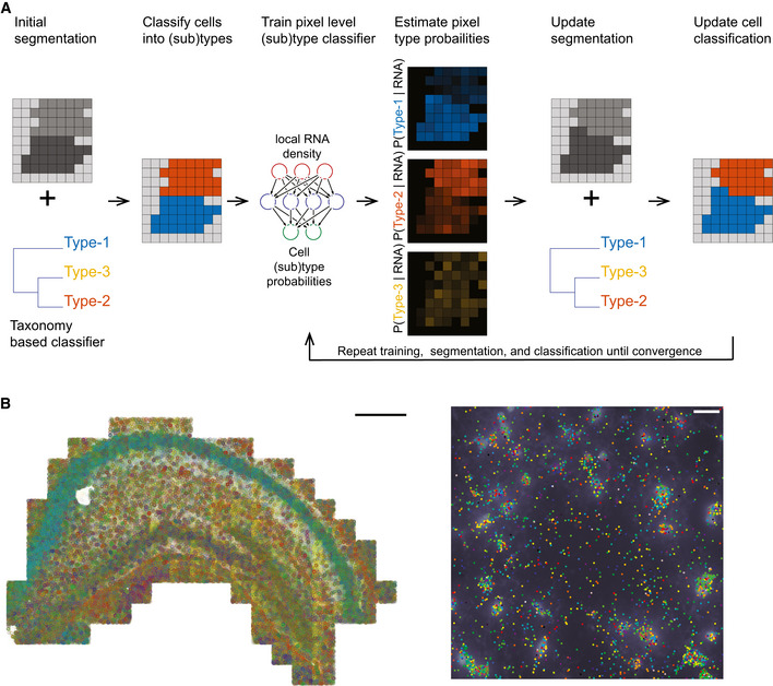
Figure 1
Overview of JSTA and the spatial transcriptomic data used for performance evaluation
Joint cell segmentation and cell type annotation (JSTA) overview. Initially, watershedu2010based segmentation is performed and a cellu2010level type classifier is trained based on the Neocortical Cell...
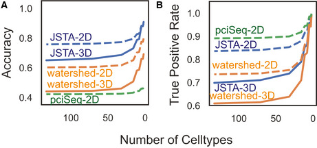
Figure EV1
Performance evaluation of JSTA, pciSeq, and watershed
A, B pciSeq is unable to run on 3D data (solid line), so we simulated additional 2D data (dotted line). We evaluated these methods on the performance of accuracy of assigning mRNA to the correct cell ...
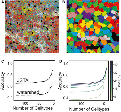
Figure 2
Performance evaluation of JSTA using simulated data
Representative synthetic dataset of nuclei (black) and mRNAs, where each color represents a different gene. Ground truth segmentation map of the cells in the representative synthetic dataset. Each col...
Figure EV2
Application of JSTA to osmFISH data from the mouse somatosensory cortex
Glutamatergic neurons are consistent with previously identified spatial patterns of the somatosensory cortex. JSTAu2010mapped highu2010resolution (sub)types are correlated with their NCTT counterparts...
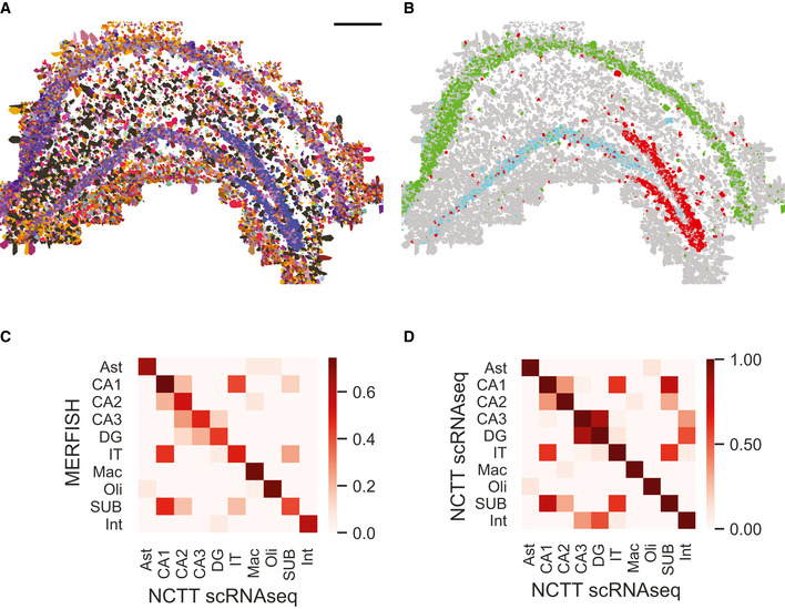
Figure 3
Segmentation of MERFISH data from the hippocampus using JSTA
Highu2010resolution cell type map of 133 cell (sub)types segmented and annotated by JSTA. Colors match those defined by Neocortical Cell Type Taxonomy (NCTT). Scale bar is 500u00a0u03bcm. JSTAu2010bas...
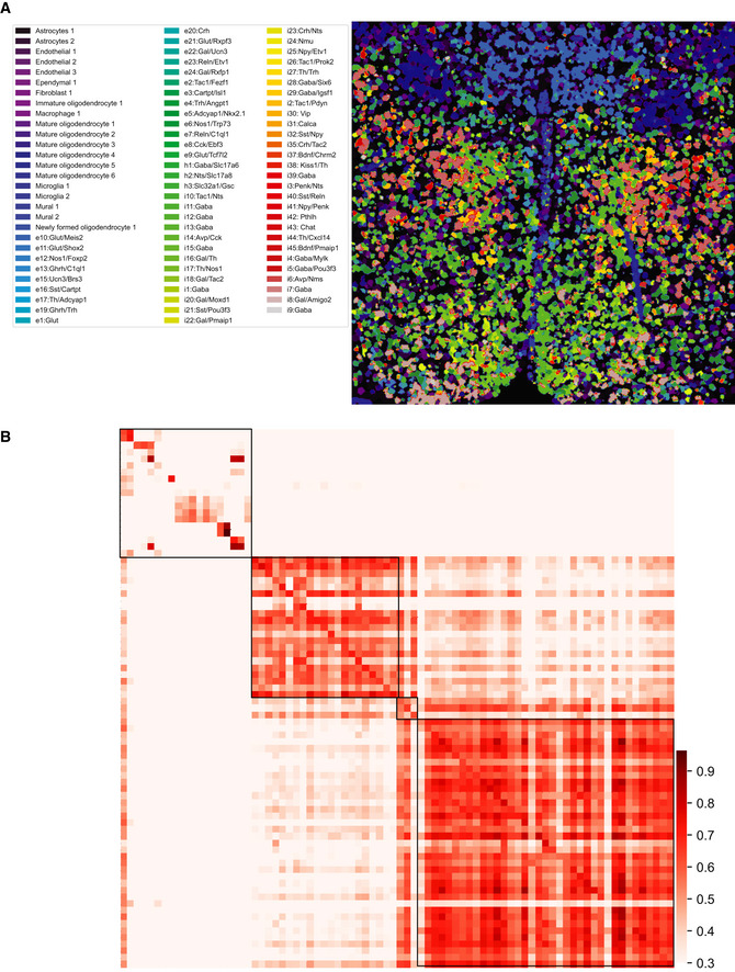
Figure EV3
Run time evaluation of JSTA on simulated data
A, B We ran JSTA on data simulated with a width and height of 100, 200, 300, 400, 500, and 1,000u00a0u03bcm, with three replicates each. We evaluated the time taken to run JSTA by the area of the sect...
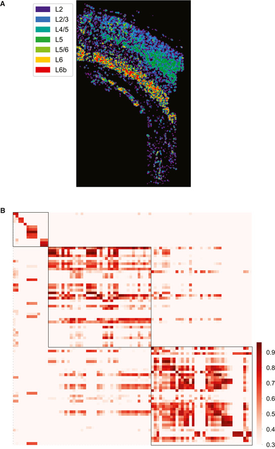
Figure EV4
Application of JSTA to MERFISH data from the mouse hypothalamic preoptic region
Highu2010resolution cell types identified by JSTA. The spatial mappings of these highu2010resolution cell types are consistent with the manually annotated data from Moffit et al (2018). JSTAu2010mappe...
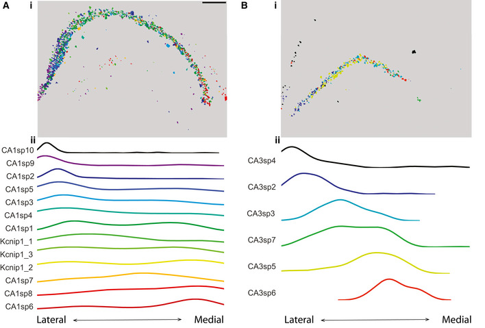
Figure 4
Spatial distribution of neuronal subtypes in the hippocampus
(i) Cell subtype map of CA1 neurons in the hippocampus as annotated by JSTA. Scale bar is 500u00a0u03bcm. Distribution of CA1 subtypes in the hippocampus, computed by projecting cell centers to the la...
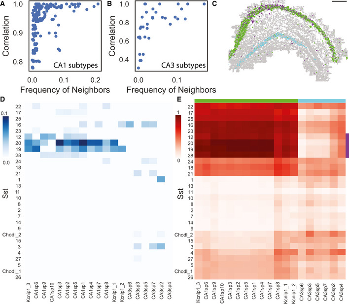
Figure 5
Agreement between spatial proximity and gene coexpression in highly granular cell subtypes in the hippocampus
A, B Relationship between the frequency of a (sub)type's neighbors and its transcriptional Pearson correlation between CA1 subtypes (A) and between CA3 subtypes (B). C Cell type map in the hippocampus...
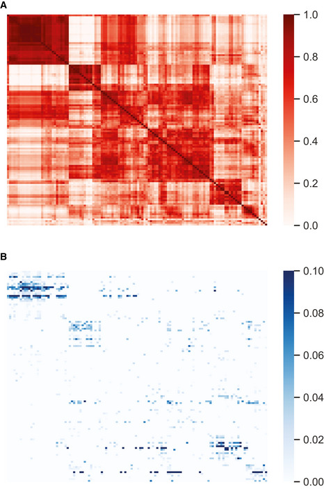
Figure EV5
Correlation structure of cell types compared with their colocalization
Neuronal subtypes that are highly colocalized are often correlated in their gene expression. Cell types with more than 10 cells were included. Pearson correlation of 122 (sub)types across 83 selected ...
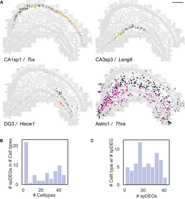
Figure 6
Identification of spatial differential gene expression (spDEGs)
Normalized expression of Tox in CA1sp1, Leng8 in CA3sp3, Hecw1 in DG3, and Thra in Astro1 shows variable expression throughout the hippocampus. Scale bar is 500u00a0u03bcm. spDEGs were computed by com...
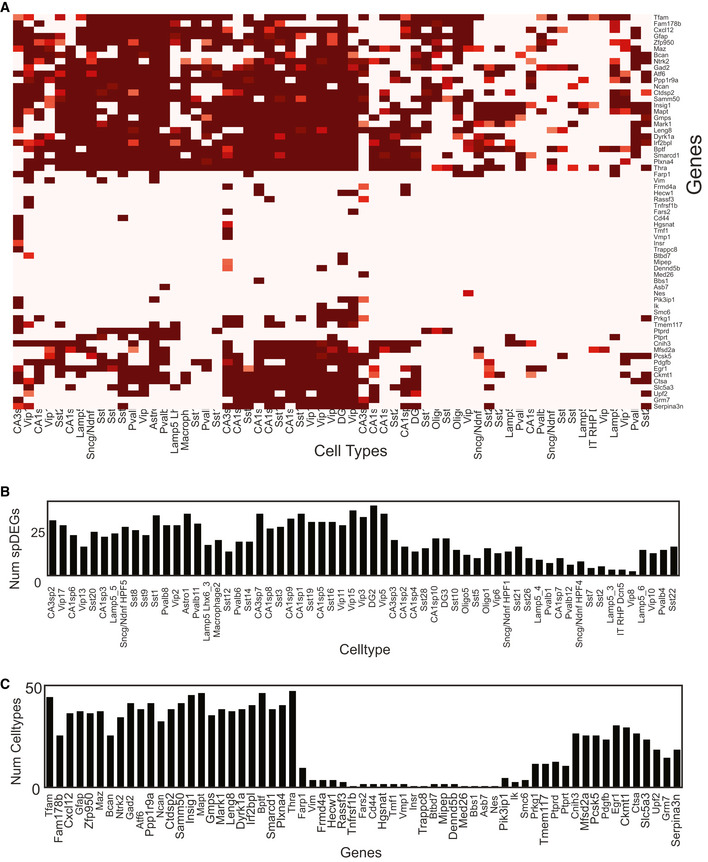
Figure EV6
Identification of spatial differentially expressed genes (spDEGs)
spDEGs were computed by comparing the true variance in gene expression between cell subtype neighborhoods to that of randomly permuted cell (sub)type neighborhoods. 63 genes across 61 cell types show ...
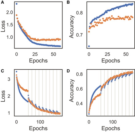
Figure EV7
Crossu2010entropy loss and accuracy of cell type (A, B) and pixel (C, D) classifier during training for the train (blue) and validation (orange) datasets
A, B Crossu2010entropy (A) loss and accuracy (B) during training cell type classifier. The cell type classifier overfits the training data and is mitigated by stopping training after 40 epochs. C, D C...
Figure images are served from the NIH/NLM PubMed Central Open Access Subset or Europe PMC; copyright remains with the publishers and authors.
💬 Discussion
0 commentsNo comments yet. Be the first to start a discussion!
Leave a Comment