Abstract
The medial prefrontal cortex (mPFC) plays a critical role in multiple cognitive and limbic functions. Given its vital importance, investigating the function of individual mPFC circuits in animal models has provided critical insight into the neural basis underlying different behaviors and psychiatric conditions. However, our knowledge regarding the mPFC whole-brain network stays largely at the anatomical level, while the functional network of mPFC, which can be dynamic in different conditions or following manipulations, remains elusive especially in awake rodents. Here we combined optogenetic stimulation and functional magnetic resonance imaging (opto-fMRI) to reveal the network of brain regions functionally activated by mPFC outputs in awake rodents. Our data showed significant increases in blood-oxygenation-level dependent (BOLD) signals in prefrontal, striatal and limbic regions when mPFC was optically stimulated. This activation pattern was robust, reproducible, and did not depend on the stimulation period in awake rats. BOLD signals, however, were substantially reduced when animals were anesthetized. In addition, regional brain activation showing increased BOLD signals during mPFC stimulation was corroborated by electrophysiological recordings. These results expand the applicability of the opto-fMRI approach from sensorimotor processing to cognition-related networks in awake rodents. Importantly, it may help elucidate the circuit mechanisms underlying numerous mPFC-related functions and behaviors that need to be assessed in the awake state.
🔬 Techniques
✨ Fluorophores
🧪 Sample Preparation
🏭 Microscope Brands
🧪 Reagent Suppliers
💻 Software Details
🏛️ Research Organizations (ROR)
Affiliated research institutions:
📋 Methods
Animals Adult male Long-Evans
(LE) rats (300–500g, Charles River Laboratories) were obtained from Charles River Laboratories. Animals were housed in Plexiglas cages (two per cage) and maintained on a 12 h light:12 h dark schedule in a room temperature of 22–24°C. Food and water were provided ad libitum . All procedures were approved by the Institutional Animal Care and Use Committee of the Pennsylvania State University.
Surgery
Each rat was anesthetized by intramuscular (IM) injections of ketamine (40 mg/kg) and xylazine (12 mg/kg). Atropine methyl nitrate (0.05 mg/kg) was injected IM to reduce bronchial secretions, and dexamethasone (0.5 mg/kg) was injected IM to prevent tissue inflammation. All rats were intubated through the oral cavity, placed in a stereotaxic frame (David Kopf Instruments, Tujunga, CA), and artificially ventilated with oxygen. Body temperature was maintained at 37°C with a heated water pad and a homeothermic heating blanket on the ventral and dorsal sides of the rat, respectively. After exposing the cranium surface, four plastic MR compatible screws (.080 × .125, nylon; PlasticsOne, Roanoke, VA) were placed along the temporal ridge. A small craniotomy was made unilaterally over the infralimbic (IL) subdivision of mPFC approximately 3 mm rostral and 0.5 mm lateral to bregma. A micropipette syringe fitted with a glass pipette tip (Hamilton Company, Reno, NV) was lowered through the craniotomy to inject 800–1200nl of AAV5.CaMKIIa.hChR2(H134R)-eYFP.WPRE.hGH (Addgene26969P, Penn Vector Core) into IL (4.4 – 4.7 mm ventral) at a rate of 60 nL/min. After the syringe was withdrawn, an optic fiber (0.4 mm diameter) embedded in a 2.5 mm ceramic ferrule (Thorlabs, 0.39 NA, Newton, NJ) was slowly advanced towards the injection site until it reached a depth of ~4.3 mm. Dental cement was applied around the screws and ceramic ferrule to create a chronic optic-fiber implant. Each rat was placed in its home cage for 3–4 weeks to allow the expression of ChR2 before starting acclimation to the MRI environment.
Show full methods section
Animals Adult male Long-Evans
(LE) rats (300–500g, Charles River Laboratories) were obtained from Charles River Laboratories. Animals were housed in Plexiglas cages (two per cage) and maintained on a 12 h light:12 h dark schedule in a room temperature of 22–24°C. Food and water were provided ad libitum . All procedures were approved by the Institutional Animal Care and Use Committee of the Pennsylvania State University.
Surgery
Each rat was anesthetized by intramuscular (IM) injections of ketamine (40 mg/kg) and xylazine (12 mg/kg). Atropine methyl nitrate (0.05 mg/kg) was injected IM to reduce bronchial secretions, and dexamethasone (0.5 mg/kg) was injected IM to prevent tissue inflammation. All rats were intubated through the oral cavity, placed in a stereotaxic frame (David Kopf Instruments, Tujunga, CA), and artificially ventilated with oxygen. Body temperature was maintained at 37°C with a heated water pad and a homeothermic heating blanket on the ventral and dorsal sides of the rat, respectively. After exposing the cranium surface, four plastic MR compatible screws (.080 × .125, nylon; PlasticsOne, Roanoke, VA) were placed along the temporal ridge. A small craniotomy was made unilaterally over the infralimbic (IL) subdivision of mPFC approximately 3 mm rostral and 0.5 mm lateral to bregma. A micropipette syringe fitted with a glass pipette tip (Hamilton Company, Reno, NV) was lowered through the craniotomy to inject 800–1200nl of AAV5.CaMKIIa.hChR2(H134R)-eYFP.WPRE.hGH (Addgene26969P, Penn Vector Core) into IL (4.4 – 4.7 mm ventral) at a rate of 60 nL/min. After the syringe was withdrawn, an optic fiber (0.4 mm diameter) embedded in a 2.5 mm ceramic ferrule (Thorlabs, 0.39 NA, Newton, NJ) was slowly advanced towards the injection site until it reached a depth of ~4.3 mm. Dental cement was applied around the screws and ceramic ferrule to create a chronic optic-fiber implant. Each rat was placed in its home cage for 3–4 weeks to allow the expression of ChR2 before starting acclimation to the MRI environment.
Optical stimulation setup
A laser (100 mW, 473 nm, Opto Engine LLC, Midvale, UT) was connected to a 7 meter long patch cable (Thorlabs, Ø400 μm core, 0.39 NA, Newton, NJ), which was attached to the optic-fiber stub implanted in the rat. The timing of the laser output was controlled by a National Instruments DAQ board (NI USB 6211, Austin, TX) with custom-written code in LabView. Light power at the end of patch cable was set at 30mW as measured by a power meter (Thorlabs, Newton, NJ). Considering power loss due to the coupling between the patch cable and the implanted fiber stub, light power at the tip of the implanted fiber was estimated approximately 15 mW. MR experiments The timeline of the experimental procedures used in this study is summarized in Figure 1 . As this figure indicates, all animals were acclimated to immobilization and the noise of the MRI scanning environment before imaging sessions were conducted using a paradigm documented in our earlier reports ( Liang et al., 2011 , 2012a , b , 2014 ; Liang et al., 2013 ; Liang et al., 2015 ; Zhang et al., 2010a ). Each animal was gradually acclimated over a 7-day period to minimize motion and the stress that accompanies imaging in the awake state ( King et al., 2005 ; Liang et al., 2014 ). Each rat was imaged twice in the awake state and then once during anesthesia, and all of these imaging sessions were separated by at least two days. For anesthetized sessions, isoflurane (1–1.5%) was delivered to the animal through a nose cone, and the respiratory rate was monitored throughout the MRI experiment. All imaging experiments were conducted on a 7T Agilent system (Agilent, Santa Clara, CA). During each MRI session, anatomical images were first acquired using a fast spin-echo multislice (fsems) sequence with the following parameters: repetition time (TR) = 2s; echo time (TE) = 40 ms; matrix size = 256×256; FOV = 3.2×3.2 cm; slice number = 20; slice thickness = 1 mm; and repetition number = 6. Gradient-echo images covering the whole brain were acquired using echo-planar imaging (EPI) with the following parameters: TR = 1 s; TE = 13.8 ms; matrix size = 64×64; FOV = 3.2×3.2 cm; slice number = 20; and slice thickness = 1 mm. We used three different paradigms—two block designs and one event-related design—for the opto-fMRI experiments. In block design 1, the laser light was alternately turned on (10Hz, 10ms pulses) for 15 s and off for 30 s with a total of three light-on periods interleaved with four light-off periods. In block design 2, the laser light was alternately turned on for 30s (10Hz, 10ms pulses) and off for 30s with three light-on periods interleaved with four light-off periods. For the event-related design, each epoch consisted of a light flash for 1s (20Hz, 10ms pulses) and an inter-stimulus interval of 30s. A total of 10 epochs were delivered for each scan. In each paradigm, light pulse delivery was triggered by a TTL signal from the MR console at the beginning of each opto-fMRI scan.
Data analysis
Anatomical images were first manually aligned to a fully segmented rat brain atlas in Medical Image Visualization and Analysis (MIVA, ccni.wpi.edu). EPI images were motion-corrected using the realign function in SPM8 ( http://www.fil.ion.ucl.ac.uk/spm/ ), and spatially smoothed (FWHM 1mm). Motion parameters were regressed out from the time course of each voxel, and then voxel time courses were linearly detrended. The first ten volumes of EPI images were discarded to allow the magnetization to reach steady state. The subsequent series of procedures for analyzing preprocessed opto-fMRI data are summarized in Figure 2 . Because the hemodynamic response function (HRF) of the optogenetically generated blood-oxygenation-level dependent (BOLD) signal is not well characterized, we adopted a Fourier analysis paradigm that does not assume a particular HRF ( Lee et al., 2010 ). For each individual voxel, the time series was Fourier transformed to the frequency domain, and the coherence value (c value) was calculated as defined in the following equation: c = ∣ F ( f 0 ) ∣ ∑ f ∣ F ( f ) ∣ 2 where | F ( f 0 )| is magnitude of the stimulation frequency component, and ∑ f ∣ F ( f ) ∣ 2 is the sum of squares of magnitudes of all frequency components. Coherence values were further converted to z values using the following equation: z = 1 σ ( c 2 ( 1 - c 2 ) ( ( N - 1 ) σ 2 + N m 2 ) - m ) where m is the mean, σ 2 is the variance, and N is the sample size for estimation of m and σ . z value images were calculated for all scans, and were subsequently averaged across individual conditions (i.e. awake or anesthetized) to yield the mean z image for each condition. To threshold the z images, we adopted an adaptive thresholding strategy developed by Allen et al. ( Allen et al., 2011 ). The distribution of z values represents a mixture of Normal and Gamma distributions. It is assumed that z values associated with optogenetic activation follow the Gamma distribution, while the remaining z values follow the Normal distribution. Thus, all z values from each mean z image were fitted by a Normal-Gamma mixture model defined as follows: p ( z ) = c ∗ N ( z ∣ μ , σ ) + ( 1 - c ) ∗ G ( z - μ ∣ α , β ) where N(.) indicates Normal distribution and G(.) indicates Gamma distribution. c , μ , and σ 2 are the proportion, mean, and variance of Normal distribution, respectively. α and β are two parameters of Gamma distribution. Five parameters ( c , μ , σ , α and β) were estimated by minimizing the residual sum of square errors between the fitted and empirical distributions using the lsqnonlin function in Matlab (Mathworks, Inc., Sherborn, MA). The fitting was separately performed on the mean z image of each condition, and the z value threshold was set based on the estimated mean and variance of Normal distribution for the condition (e.g. a threshold of z > μ + 3 σ corresponds to a p value of 0.001 for mean z images). To statistically compare the BOLD activation maps between the awake and anesthetized conditions, a linear mixed effect model (implemented in fitlme function in Matlab) was applied to z-value maps of all sessions with conditions (awake or anesthetized) as the fixed effect and animals as the random effect. For each individual voxel, a t value and p value were generated, and p
📊 Figures

Figure 1
Schematic diagram illustrating the timeline of the experiment paradigm.
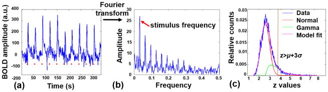
Figure 2
Procedures for analyzing opto-fMRI data. Left, a representative BOLD time course in response to ten 1-second stimuli delivered at the rate of one stimulus per 30 seconds (red triangles). Middle, the p...
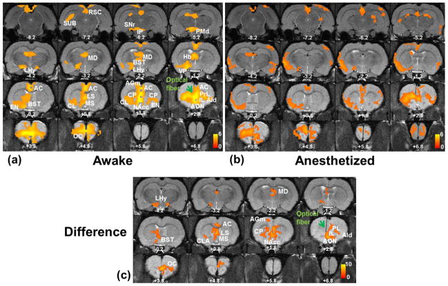
Figure 3
Averaged activation maps in response to IL optogenetic stimulation. a) The averaged activation map in the awake state. b) The averaged activation map in the anesthetized state. Both maps in a) and b) ...
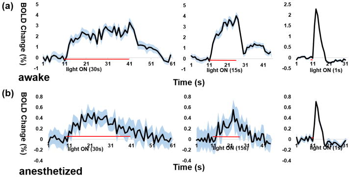
Figure 4
Time courses of optically-evoked BOLD signals in the anterior cingulate (AC) cortex during awake and anesthetized states. a) Time courses in the awake state. b) Time courses in the anesthetized state....
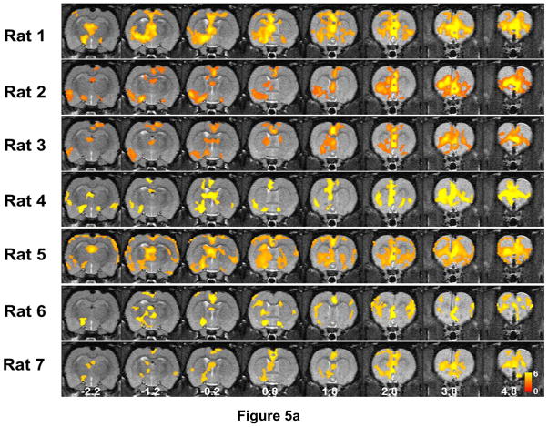
Figure 5
a) Activation maps of all individual rats in the awake state. For each rat, two awake sessions were averaged. Maps were thresholded at z > u03bc + 2 u03c3 (i.e. p<0.05 at the whole brain level). Di...
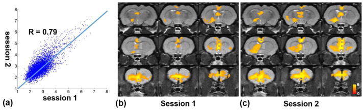
Figure 6
Consistent activation maps between the first and second awake imaging sessions. a) The voxel-wise correlation of z values between the two awake sessions averaged across all rats. b) The averaged activ...
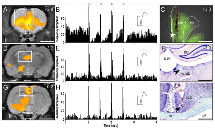
Figure 7
Photo-stimulation of IL increases neuronal discharges in areas of increased BOLD signaling in the IL network. A, D, and G: Mean BOLD signal change across rats after photo-stimulating IL. White boxes i...
Figure images are served from the NIH/NLM PubMed Central Open Access Subset or Europe PMC; copyright remains with the publishers and authors.
💬 Discussion
0 commentsNo comments yet. Be the first to start a discussion!
Leave a Comment