Abstract
Information processing is energetically expensive. In the mammalian brain, it is unclear how information coding and energy use are regulated during food scarcity. Using whole-cell recordings and two-photon imaging in layer 2/3 mouse visual cortex, we found that food restriction reduced AMPA receptor conductance, reducing synaptic ATP use by 29%. Neuronal excitability was nonetheless preserved by a compensatory increase in input resistance and a depolarized resting potential. Consequently, neurons spiked at similar rates as controls but spent less ATP on underlying excitatory currents. This energy-saving strategy had a cost because it amplified the variability of visually-evoked subthreshold responses, leading to a 32% broadening of orientation tuning and impaired fine visual discrimination. This reduction in coding precision was associated with reduced levels of the fat mass-regulated hormone leptin and was restored by exogenous leptin supplementation. Our findings reveal that metabolic state dynamically regulates the energy spent on coding precision in neocortex.
🔬 Techniques
🔭 Microscopes
🧬 Organisms
💻 Software
✨ Fluorophores
🧪 Sample Preparation
🔬 Cell Lines
🏭 Microscope Brands
🧪 Reagent Suppliers
📷 Detectors
🔎 Objectives
💻 Software Details
💻 Code & Software
💾 Data Repositories
🏷️ Research Resource Identifiers (RRIDs)
Verified research resources used in this paper:
🏛️ Research Organizations (ROR)
Affiliated research institutions:
📋 Methods
Key resources table REAGENT or RESOURCE SOURCE IDENTIFIER
Bacterial and virus strains AAV1.Syn.Flex.GCaMP6s.WPRE.SV40 Addgene RRID:Addgene_100845-AAV1 AAV1.CamKII 0.4.Cre.SV40 AAV1 Addgene RRID:Addgene_105558-AAV1 Chemicals, peptides, and recombinant proteins Recombinant Murine Leptin Peprotech, UK Cat#AF-450-31 Critical commercial assays Mouse Leptin Quantikine Elisa Kit R&D Systems, USA Cat#MOB00B Deposited data Custom MATLAB scripts for data analysis and computational models This paper https://github.com/rochefort-lab/Padamsey-et-al-Neuron-2021 ; https://doi.org/10.5281/zenodo.5561795 Experimental models: Organisms/strains Mouse: C57BL/6J The Jackson Laboratory RRID: IMSR_JAX:000664 Mouse: B6-Tg(Thy1.2-ATeam1.03 YEMK ) AJhi Prof. Dr. Johannes Hirrlinger, Carl-Ludwig-Institut for Physiology RRID: MGI:5882597 Software and algorithms MATLAB 2013/2017a Mathworks RRID: SCR_001622 Psychophysics Toolbox package for MATLAB http://psychtoolbox.org RRID: SCR_002881 SIMA 1.3.2 (sequential image analysis) ( Kaifosh et al., 2014 ) https://pypi.org/project/sima/ FISSA ( Keemink et al., 2018 ) https://github.com/rochefort-lab/fissa ImageJ (Fiji) NIH – public domain https://fiji.sc ; RRID: SCR_002285 Custom MATLAB scripts for data analysis and computational models This paper https://github.com/rochefort-lab/Padamsey-et-al-Neuron-2021 https://doi.org/10.5281/zenodo.5561795 WinWCP Strathclyde Electrophysiology Software RRID: SCR_014713 pCLAMP10 Molecular Devices RRID: SCR_011323 ANY-maze Stoelting, Europe RRID: SCR_014289 Resource availability Lead contact Further information and requests for resources and materials should be directed to and will be fulfilled by the lead contact Nathalie L. Rochefort ( n.rochefort@ed.ac.uk ).
Show full methods section
Key resources table REAGENT or RESOURCE SOURCE IDENTIFIER
Bacterial and virus strains AAV1.Syn.Flex.GCaMP6s.WPRE.SV40 Addgene RRID:Addgene_100845-AAV1 AAV1.CamKII 0.4.Cre.SV40 AAV1 Addgene RRID:Addgene_105558-AAV1 Chemicals, peptides, and recombinant proteins Recombinant Murine Leptin Peprotech, UK Cat#AF-450-31 Critical commercial assays Mouse Leptin Quantikine Elisa Kit R&D Systems, USA Cat#MOB00B Deposited data Custom MATLAB scripts for data analysis and computational models This paper https://github.com/rochefort-lab/Padamsey-et-al-Neuron-2021 ; https://doi.org/10.5281/zenodo.5561795 Experimental models: Organisms/strains Mouse: C57BL/6J The Jackson Laboratory RRID: IMSR_JAX:000664 Mouse: B6-Tg(Thy1.2-ATeam1.03 YEMK ) AJhi Prof. Dr. Johannes Hirrlinger, Carl-Ludwig-Institut for Physiology RRID: MGI:5882597 Software and algorithms MATLAB 2013/2017a Mathworks RRID: SCR_001622 Psychophysics Toolbox package for MATLAB http://psychtoolbox.org RRID: SCR_002881 SIMA 1.3.2 (sequential image analysis) ( Kaifosh et al., 2014 ) https://pypi.org/project/sima/ FISSA ( Keemink et al., 2018 ) https://github.com/rochefort-lab/fissa ImageJ (Fiji) NIH – public domain https://fiji.sc ; RRID: SCR_002285 Custom MATLAB scripts for data analysis and computational models This paper https://github.com/rochefort-lab/Padamsey-et-al-Neuron-2021 https://doi.org/10.5281/zenodo.5561795 WinWCP Strathclyde Electrophysiology Software RRID: SCR_014713 pCLAMP10 Molecular Devices RRID: SCR_011323 ANY-maze Stoelting, Europe RRID: SCR_014289 Resource availability Lead contact Further information and requests for resources and materials should be directed to and will be fulfilled by the lead contact Nathalie L. Rochefort ( n.rochefort@ed.ac.uk ).
Materials availability
This study did not generate new unique reagents.
Experimental model and subject details
All animal experiments were approved by the Animal Welfare and Ethical Review Board (AWERB) of the University of Edinburgh and were performed under a project license granted by the UK Home Office and conformed with the UK Animals (Scientific Procedures) Act 1986 and the European Directive 86/609/EEC and 2010/63/EU on the protection of animals used for experimental purposes. This study used male C57BL/6J mice (RRID:IMSR_JAX:000664; Jackson Laboratory) and male B6-Tg (Thy1.2-ATeam1.03 YEMK ) AJhi transgenic mice on a C57BL/6J background (RRID:MGI:5882597; https://scicrunch.org/resources ). Animals were group housed (2-5/cage) in a reverse 12h/12h light/dark cycle room that was kept at 21 ± 2°C and 55 ± 10% humidity. Mice 7-9 weeks of age either had ad libitum access to food (RM1 expanded pellets for maintenance; DBM Scotland UK) or were food-restricted to 85% of their baseline bodyweight (calculated from a three-day average) for a minimum of 2 weeks prior to experimentation and maintained at this bodyweight for the duration of the experiment (experimental duration: in vivo electrophysiology: 1 day; imaging; 1-3 weeks; behavior: 4-8 weeks). Food-restricted animals were given one ration of food 4-8 hours prior to the end of their dark cycle. At the start of food restriction, the food rations started at 4-5g/animal, which was in excess of daily ad libitum consumption, and was systematically reduced by at most 20%/day until animals achieved 85% of their baseline bodyweight. Both control and food-restricted animals were handled and weighed daily. Unless otherwise specified, animals were given ad libitum access to food for 1-3 hours prior to experimentation in order to state them Food-restricted animals typically required 45-90 minutes to satiate, as evidenced by no observable feeding for 10 minutes, and never consumed more than 80% of their allocated daily food weight during this time. The consumed weight of food was deducted from the day’s allocated ration of food, which was given at the regular feeding time. For behavioral experiments, animals were tested after they consumed their daily ration of food. Method details AAV injection and cranial window Mice were anesthetized during surgery using isoflurane and maintained at 37°C using a servo-driven heater. They were given buprenorphine (Vetergesic; 0.1 mg/kg), carprofen (Carprieve, 5 mg/kg), and dexamethasone (Rapidexon, 2 mg/kg) subcutaneously pre-operatively, and 25mL/kg of warm Ringer’s solution subcutaneously at the end of the surgery. Non-transparent eye cream was applied to protect the eyes (Bepanthen, Bayer, Germany) during surgery. A square craniotomy (2 × 2 mm) was made over the left primary visual cortex with its center at 2.5 mm mediolateral and 0.5 mm anterior to lambda. A flexed variant of GCaMP6S (AAV1.Syn.Flex.GCaMP6s.WPRE.SV40; 1:10 dilution in saline; Addgene; RRID:Addgene_105558-AAV1) along with Cre-recombinase under the CaMKII promoter (AAV1.CamKII 0.4.Cre.SV40; 1:100 dilution in saline; Addgene; RRID:Addgene_105558-AAV1) was injected at the center of the craniotomy. A total of 50 nL of virus solution was injected at each of 3 depths (150, 250 and 350 μm), via a sharp glass pipette, at a rate of 2.5 nL / 30 s using a Nanoject II (Drummond Scientific). Injections started at the deepest site. At least 5 minutes elapsed after the complete injection of 50 nL before moving to another depth. The craniotomy was then covered with a square glass window, which was superglued in place. The window consisted of 2 glass coverslips (Menzel-Glaser # 0) glued together with optically-clear, UV-cured glue (Norland Optical Adhesive no. 60); the inner window was 2.0 mm x 2.0 mm, the outer window was 2.5 mm x 2.5 mm. A custom metal headplate was superglued on to the skull and fixed with dental cement (Paladur, Heraeus Kuzler). Imaging sessions were performed 2-4 weeks after viral injection. Habituation and head-fixation Mice were extensively handled (daily for 2-3 weeks) and habituated to the cardboard tube used for the recordings. In addition, mice were exposed to cardboard tubes in their home cage that were similar to the one present on the experimental rig. During imaging or electrophysiological recordings, mice were placed in a similar cardboard tube and head-fixed. The cardboard tube was positioned on top of a Styrofoam wheel (20 cm diameter). For calcium imaging, mice were habituated to head-fixation prior to experimentation in a once daily, 10-15 minute session for 2 days. For ATP imaging and electrophysiological recordings, mice were habituated to the imaging setup without head fixation (10-15 min session/day for 1-2 days). We found that mice quickly became accustomed to the setup, evident by the absence of resistive movements and the presence of occasional grooming behaviors, and remained stationary within the tube ( Figure S2 B).
Pupil and movements tracking
We used an optical encoder (E7P, 250cpr, Pewatron, Switzerland), to monitor movements of the Styrofoam wheel throughout imaging and recording sessions. Movements associated with the mouse visibly adjusting its posture were readily detected in this way. Pupil dilation was also monitored in some experiments using a camera (30 frames/s; USB 2.0 monochrome camera; ImagingSource). In vivo two-photon imaging ATP and calcium imaging were performed using a custom-built resonant scanning two-photon microscope, as described previously ( Henschke et al., 2020 ; Pakan et al., 2016 , 2018 ). The setup was equipped with a Ti:Sapphire laser (Charmeleon Vision-S, Coherent, CA) and GaAsP photomultiplier tubes (Scientifica). Images were acquired using a 25x water-immersion objective (Nikon; CF175 Apo 25XC W; 1.1 NA) at a rate of 40 Hz using a custom-programmed LabView based software (v8.2; National Instruments, UK). Time-series images of one focal plane per mouse were acquired, imaged at depths between 160 and 280 μm below the pia. For GCaMP6s imaging, excitation was tuned to 920nm. Visual stimuli Visual stimuli were generated using MATLAB (Mathworks; RRID: SCR_001622 ; Psychophysics Toolbox; RRID: SCR_002881 ) and displayed on an LCD monitor (51 × 29 cm; Dell) at a distance of 20 cm from the eye, contralateral to the hemisphere with the cranial window. For a given trial, 12 drifting gratings with angles ranging from 0 – 330° (30° increments) were presented in random order. Each grating was presented with a temporal frequency of 1 Hz for 2 s. Gratings within a trial had the same spatial frequency. For calcium imaging, gratings across trials were randomly assigned a spatial frequency (0.02, 0.04, 0.16, or 0.32 cpd). For electrophysiological recordings, a spatial frequency of 0.04 cpd was used for all gratings. Gratings were interspersed with the presentation of a gray screen (4 s for imaging and 1 s for electrophysiology experiments). All trials started and ended with the presentation of a black screen (4 s for imaging and 1 s for electrophysiology experiments). For natural stimuli, we either used a movie of the outdoors (filmed at a nearby park) or a movie taken inside the home cage of a group of mice (5 animals) from within the animal house. Movie presentations lasted 60 s for imaging experiments and 35 s for electrophysiology experiments. In vivo ATP imaging We used a transgenic mouse line B6-Tg(Thy1.2-ATeam1.03 YEMK ) AJhi that expressed the FRET-based ATP sensor ATeam1.03 YEMK under the Thy1.2 promoter ( Trevisiol et al., 2017 ) (RRID:MGI:5882597; https://scicrunch.org/resources ). On the day of experimentation, a given animal was anesthetized with isoflurane gas and administered carprofen (Carprieve, 5 mg/kg), along with 25 mL/kg of warm Ringer’s solution subcutaneously. A custom metal headplate was first superglued on to the skull and fixed with dental cement (Paladur, Heraeus Kuzler). A small cranial window (∼0.5 x ∼0.5 mm) was then made above the left visual cortex and covered with a 4% agarose solution, followed by application of silicone to ensure a good seal. The dura was kept intact. The animal was allowed to recover (30-60 minutes) prior to being head-fixed and imaged, during which time the silicone and agarose were removed and replaced with HEPES-buffered ACSF (in mM: 124 NaCl, 20 Glucose, 10 HEPES, 2.5 KCl, 1.2 NaH 2 PO 4 , 2 CaCl 2 , and 1 CaCl 2 ; pH 7.2-7.4). For two-photon imaging, the laser was tuned to 850 nm for excitation. CFP and YFP fluorescence were recorded simultaneously using a 515nm long-pass dichroic mirror with 485/70nm (CFP) and 535/45nm (YFP) emission filters (mirror and filter set: T515lpxr C156624; Scientifica). Imaging was performed during the presentation of an outdoor movie (60 s/trial). Three trials were taken at baseline, after which ATP synthesis inhibitors (1 mM oligomycin and 20 mM sodium iodoacetate) were added to the ACSF to isolate ATP usage. Thirty trials were successively performed immediately after drug application. We confirmed that there were no differences between control and food restricted groups in FRET decay with drug application alone, in the absence of visual stimulation (FRET decay in CTR group versus FR group; −0.084 ± 0.003/s versus −0.080 ± 0.005/s; t test: p = 0.56; n = 8 CTR and 6 FR animals) In vivo electrophysiology On the day of experimentation, a given animal was anesthetized with isoflurane gas and administered carprofen (Carprieve, 5 mg/kg), along with 25 mL/kg of warm Ringer’s solution subcutaneously. A custom metal headplate was first superglued on to the skull and fixed with dental cement (Paladur, Heraeus Kuzler). Following, a small cranial window (no more than 0.5 × 0.5 mm) was made above the left visual cortex and covered with a 4% agarose solution, followed by application of silicone to ensure a good seal. The dura was kept intact. The animal was allowed to recover (30-60 minutes) prior to being head-fixed and imaged, during which time the silicone and agarose were removed and replaced with HEPES-buffered ACSF. Patch recordings were obtained using a Multiclamp 700B (Molecular Devices) amplifier and WinWCP software (University of Strathclyde Glasgow). Data were acquired at 20 kHz and filtered at 3 kHz using a digitizer (Digidata 1440, Axon Instruments). Borosilicate patch electrodes (4-6 MΩ; 1.5 mm outer diameter; 0.86 mm inner diameter; Harvard apparatus) were pulled to have a long taper using a two-step pull on a Narashige vertical puller (PC-100) and were filled either with a potassium-based internal solution for current clamp recordings (in mM: 130 Kgluconate, 10 KCl, 10 HEPES, 2 Na 2 ATP, 0.4 Na 3 GTP, 2 MgCl 2 , and 0.3 EGTA; pH 7.2-7.4) or a cesium-based internal solution for voltage-clamp recordings (in mM: 140 CsMeSO 4 , 10 HEPES, 2 Na 2 ATP, 0.4 Na 3 GTP, 2 MgCl 2 , 0.3 EGTA, 5 QX314-Cl and 5 TEA-Cl; pH 7.2-7.4). In vivo blind patch recordings were made as previously described ( Adesnik, 2017 ; Brown et al., 2019 ). Electrodes were placed in the bath and advanced with a positive pressure (300 mBar) at a 45° angle using a microdrive (Scientifica) while electrode resistance was monitored. Electrode depth was zeroed upon a sudden increase in resistance, which indicated contact with the dura. The electrode was rapidly advanced by ∼100 μm to break the dura; electrodes were discarded if resistance did not rapidly return to within 5% of its original value. After successful penetration, the electrode was advanced to 150 μm below the pia surface and positive pressure was reduced to 20-30 mBar. The pipette was then slowly advanced in 2 μm steps. A bounce-like increase in resistance in response to each of 3 successive steps indicated contact with a putative cell, at which point positive pressure was released and a gigaohm seal was attempted by applying slight negative pressure if necessary. Electrodes were discarded on failed attempts, or if no cell was encountered within 350 μm of the pia surface. Following formation of a gigaohm seal, negative pressure was used to break-in. Whole-cell recording (20-40 MΩ) was subsequently optimized by applying slow negative or positive pressure. Pipette capacitance was fully compensated. The quality of recording was constantly monitored using a negative current or voltage step. Only neurons with stable series resistance were used (< 20% change throughout the recording). The liquid junction potential was not corrected. Excitatory and inhibitory currents were recorded at −70 mV and +10 mV. In experiments assessing voltage-dependent subthreshold variability, the resting membrane potential was hyperpolarized by injecting hyperpolarizing current (−50pA to −100pA) of sufficient magnitude to prevent spiking during grating presentations. We obtained current clamp recordings from a total of 33 control and 26 food-restricted animals, and voltage-clamp recordings from a total of 13 control and 10 food-restricted animals.
Ex vivo electrophysiology
Acute slices were prepared from the visual cortex. The brain was extracted and coronally sectioned (400 μm thick) in ice-cold dissection media (in mM: 87 NaCl, 75 sucrose, 2.5 KCl, 25 NaHCO3, 1.25 NaH2PO4, 25 glucose, 0.5 CaCl2, 7 MgCl2; 95% O 2 , 5% CO 2; pH 7.2-7.4) using a vibratome (VT1200s, Leica, Germany). Slices containing V1 were isolated and allowed to recover for 30–60 minutes in heated (35°C) ACSF (in mM: 125 NaCl, 2.5 KCl, 25 NaHCO3, 1.25 NaH2PO4, 25 glucose, 2 CaCl2, 1 MgCl2; 95% O 2 , 5% CO 2; pH 7.2-7.4) before being stored at room temperature. During recordings, slices were perfused with heated (33°C) ACSF (6-8 mL/minute). Cells were visualized with IR-DIC illumination (BX-51; Olympus), first with a 4x objective lens (0.1 N.A.; Olympus), and then with a 20x water-immersion lens (1.0 N.A.; Olympus). Layer 2/3 pyramidal cells were patched with borosilicate glass electrodes (4–7 MΩ) pulled on a horizontal electrode puller (P-97 Sutter Instruments). Electrodes were filled either with a potassium-based internal solution for current clamp recordings or a cesium-based internal solution for voltage-clamp recordings. Cellular electrophysiology was recorded using a Multiclamp 700B amplifier and associated pCLAMP 10.0 software (Molecular Devices). Data were acquired at 20 kHz and filtered at 3 kHz using a digitizer (Digidata 1440, Axon Instruments). Pipette capacitance was compensated. Series resistance was < 20MΩ. Only neurons with stable series resistance were used (< 20% change throughout the recording). The liquid junction potential was not corrected. Excitatory currents were recorded at −70 mV. Evoked currents were triggered using a glass stimulating electrode coupled to a constant current stimulator (Digitimer). The electrode was placed in layer 2/3, 50-100 μm from the patched cell body, perpendicular to the long axis of the apical dendrite. A minimum of 5 trials were conducted at each stimulation intensity, with a 1 s baseline recording before stimulation and 15 s between each stimulation trial. Stimulation intensity was normalized to the mean threshold intensity required to evoke an EPSC in neurons of slices from control animals. Stimulus intensity was re-normalized each time the stimulation electrode was changed. The same stimulation electrode was used for slices from at least one control and one food-restricted animal, in randomized order. Paired-pulse stimulation consisted of two stimulation pulses delivered 70 ms apart. A minimum of 5 paired-pulse trials were conducted, 30 s apart. Miniature EPSC recordings were recorded at −70 mV for a minimum of 10 minutes/cell in the presence of 1 μM TTX. Forced-choice visual discrimination task for assessing visual discrimination Mice were trained in a two-alternative forced-choice visual discrimination task ( Wong and Brown, 2006 ). Mice were placed in a trapezoid-shaped pool (140 cm long x 80 cm wide x 40 cm high; ∼22°C), filled with opaque water (liquid latex; Palace chemicals, Liverpool, UK). A 56 cm divider was placed perpendicular to the wider end of the pool to form 2 arms. Extra-maze cues were obscured by a white curtain. Mice had to locate a platform (10 cm diameter) that was kept invisible (∼2 cm submerged) in front of a specific visual cue (grating of specific orientation and direction present in one of the two arms). Visual stimuli were displayed on two identical computer monitors (1920 × 1080 pixels; 22-inch TK410V, LG) placed at water level at the larger side of the trapezoid pool, one associated with each arm, behind a transparent plexiglass wall (55 cm high). Visual cues of square-wave gratings (1 Hz, contrast 80%, 0.03 cpd, as seen from the edge of the platform) or an isoluminant gray screen were generated through the psychophysics toolbox (MathWorks). A black curtain was added behind the monitors to provide additional directionality, and the visible cue was removed from the escape platform. Mice were tested in three phases. First, mice were trained for 3 days with a visible platform (a visible cue was placed on top of the hidden platform) (pretraining; 4 trials/day, 15 min intertrial interval (ITI)). All mice decreased their latency to find the visible platform over three days; there was no difference between food groups (Two-way Repeated-measures ANOVA ; CTR group versus FR group; p = 0.58; n = 13 CTR and 15 FR animals). In the second phase (visual detection; 10 trials/day, 6 days, 15 min ITI), mice were trained to swim to a hidden platform placed in the arm associated with a vertically oriented drifting grating (90°; target stimulus); the other computer screen displayed a uniform gray stimulus (non-target stimulus). The arm with the vertical grating and platform was randomized in each trial. Each trial lasted a maximum of 90 s; mice failing to find the platform were guided to the platform. If the mouse crossed the imaginary line running perpendicular to the end of the 56 cm divider (decision line) on the wrong (non-target) stimulus side, then the trial was recorded as an error, and after finding the platform, the mouse was returned immediately to the release location to perform another trial until the mouse made a correct choice or for a maximum of 3 consecutive trials. An error trial also occurred if the mouse failed to reach any platform position within 90 s. Only mice that showed over 70% performance (averaged across 2 days) were used for the next phase. In the third phase (pattern discrimination; 10 trials/day, 9 days, 15 min ITI), mice were trained to swim to the hidden platform placed in front of the computer screen with a vertically oriented drifting grating (90°, target stimulus) versus a 45° oriented drifting grating (non-target stimulus). All other aspects of pattern discrimination training followed the procedure of visual detection training. In the final phase of the experiment, mice were tested for their visual discrimination threshold by reducing the angle difference between the vertically oriented drifting grating (target stimulus) and the non-target stimulus. The following angle differences were tested: 30° (90° versus 60°; 10 trials/day, 2 days), 20° (90° versus 70°; 10 trials/day, 2 days), 10° (90° versus 80°; 10 trials/day, 2 days), 7.5° (90° versus 82.5°; 10 trials/day, 2 days), 5° (90° versus 85°; 10 trials/day, 1 day). At the end of visual perception testing, true chance was assessed by testing 4-10 trials of 0° angle difference (90° versus 90°). Finally, mice were also re-assessed in discriminating 90° versus 45° (10 trials/day, 1 day) to confirm their ability to discriminate patterns at the end of the testing experiment; both groups retained > 70% criterion performance (CTR performance: 82.31 ± 3.42%; n = 13 animals; FR performance: 78.00 ± 2.62%; t test; p = 0.32; n = 15 CTR and FR animals). All mice remained on the platform for 15 s before being removed from the pool. Platform locations were pseudorandomized across trials and counterbalanced across mouse groups. Release location was the same throughout all phases. Between trials, mice were dried with a towel and were returned to a holding cage (similar to their home cage), which was placed on a heating pad with monitored temperature. A video camera mounted above the pool recorded the sessions for offline analysis. Leptin supplementation Leptin levels were supplemented by twice daily intraperitoneal injections of mouse recombinant leptin (Peprotech, UK; 12.5 μg/g dissolved in saline delivered at 09:00 and 18:00; adapted from ( Halaas et al., 1995 )) for 10 days; controls received saline.
Serum collection and analysis
Serum glucose, β-hydroxybutyrate, adrenaline, corticosterone and leptin levels were assayed using colorimetric detection kits as per manufacturer’s instructions (Glucose Colorimetric Detection Kit, ThermoFisher Scientific, UK; Ketone Body Colorimetric Assay Kit, Cayman Chemical, USA; Adrenaline ELISA Kit, BioVision, USA; Corticosterone Parameter Assay, R&D Systems, US; Mouse Leptin Quantikine Elisa Kit, R&D Systems, USA). Trunk blood was collected between 16:00-19:00 from animals that were briefly anesthetized with isoflurane prior to being decapitated. Blood was allowed to clot for 1-2 hours then centrifuged for 20 minutes at 2000 x g; the serum was drawn off and stored at −80°C until used. For sample collection from sated, food restricted animals, animals were first sated with ad libitum access to food for 1-3 hours prior to blood collection; food restricted animals were otherwise unfed (unsated). Animals being supplemented with leptin or saline had their injections at least 9 hours prior to sample collection. Hodgkin-Huxley type model neuron Numerical simulations were performed using the NEURON simulation environment ( Hines and Carnevale, 1997 ) interfaced with Python ( Hines et al., 2009 ). Custom channels were defined using NEURON’s Channel Builder. Analysis was done in Python, channel calibration in MATLAB. Code is available on the github repository (custom channels, script simulation, and analysis). The behavior of the membrane was represented by a simple electrical circuit, following the work of ( Hodgkin and Huxley, 1952 ). For simplicity we used the standard single compartment model, which includes a capacitive current, a leakage current with passive conductance independent of membrane voltage, and the two ionic currents sodium (Na v ) and potassium (K v ), which account for action potential dynamics, with voltage-dependent conductances ( Tables S1 and S2 ). For the Na v channel kinetics, we used the Markov model with an allosteric relationship between activation and inactivation described in ( Carter et al., 2012 ). For the delayed rectifier K v current, we used the channel described by ( Hodgkin and Huxley, 1952 ) but with faster kinetics, as in( Hansel and Sompolinsky, 1996 ) and ( Wang and Buzsáki, 1996 ). The kinetics, maximal conductances, and voltage dependency of channels were adjusted to obtain action potentials with spike threshold and shape similar to those observed in cortical neurons. Conductances were close to values previously published in single compartments models ( Golomb et al., 2006 ; Wang and Buzsáki, 1996 ); a low K v conductance was necessary for a brief afterhyperpolarization. Despite the fact that Na v and K v channels in our model contributed to subthreshold membrane depolarization, their fast gating kinetics lead to small fluctuations, which initiated spontaneous spiking over a very limited range of input in our system (see ( O’Donnell and van Rossum, 2014 ) for a detailed analysis of the contributions of stochastic Na v and K v channels). Therefore, we added a slower-activating channel so as to introduce larger subthreshold fluctuations. For simplicity, we used the original Hodgkin-Huxley K v channel, which has been well characterized and was shown to be the dominant source of membrane noise in the Hodgkin-Huxley model ( O’Donnell and van Rossum, 2014 ; Steinmetz et al., 2000 ). The conductance was adjusted to get an appropriate level of noise without significantly affecting AP dynamics. Finally, input resistance R = 1 / g L and membrane capacitance C m were set so that the membrane time constant was τ = C m / g L = 10 ms. Leak reversal potential was set to maintain the desired membrane potential at rest. All parameter values are summarized in Supplemental Tables S1 and S2 .
Model parameters
We simulated the two main features observed in food restriction by 1) dropping the leak conductance g L (inverse input resistance) to 79% of the control value, and 2) increasing the leak reversal potential E L by +5 mV, thus depolarizing the resting membrane potential. We used the same channel models in both conditions, and thus the voltage dependency of the ionic currents was the same across groups. We also ran the simulations for two intermediate conditions, namely increased input conductance alone and depolarized membrane resting potential alone. See Table S1 for a summary of the four groups. Synaptic input Synaptic input conductance was simulated as a single large event, similar to ( Liu et al., 2011 ), and was defined as g ( t ) = g p e a k × f × ( e − t / τ d e c a y − e − t / τ r i s e ) , where τ r i s e and τ d e c a y are the synaptic rise and decay time constants, set to 70 ms and 75 ms respectively. The factor f normalizes the peak of the exponential term to 1 and is automatically computed within the class Exp2Syn in the NEURON simulator. We only included an excitatory synapse (AMPAR) with reversal potential equal to 0 mV. In the remaining text, when we mention synaptic conductance we refer to the peak conductance g p e a k . For each group, we determined the minimal synaptic conductance that triggered exactly one action potential, which we refer to as rheobase conductance, noted g 0 grou p .
Table
S1 gives the rounded values of the synaptic compensation g 0 group /g 0 control . External and intrinsic noise Two noise models were used to induce trial-to-trial variability ( Figure 5 ), which differed depending on whether noise was generated by an external source or intrinsically. We modeled the external source of noise by injecting a different conductance at each trial. For a given average synaptic input g ¯ , we sampled a conductance from a normal distribution with mean g and standard deviation σ that scaled proportionally with g ¯ . If we note σ 0 the standard deviation for the control group at rheobase conductance g 0 control , variability was then scaled for each group ( Table S1 ) by a factor ρ such that σ = ρ × σ 0 , where ρ = g ¯ / g 0 group . The standard deviation σ 0 was set to approximately match the level of fluctuations observed with stochastic channels. For the intrinsic noise model, intrinsic variability was simulated with stochastic ion channels, thus noise was voltage-dependent. Only the subthreshold channel was stochastic, while Na v and K v were kept deterministic. The surface area was 200 μm 2 .
Simulations and analysis
For each group and noise model, we varied the input conductance proportionally to rheobase and recorded the probability of generating at least one spike. The data was fitted with a generalized logistic model. For the input-output curves shown in Figure 5 , we took an interval up to rheobase conductance and scaled the response to its maximum value. We then generated a set of synaptic conductances from a Gaussian tuning curve (parameters: amplitude = 0.9; width = 170°) and using the fitted input-output curve we inferred the spike output probability. We fitted a Gaussian curve to the normalized spike probability. To quantify the level of trial-to-trial variability in the system, we measured the maximum depolarization at each trial (97.5 th quantile) after clipping the AP, and computed the CV as the ratio between the standard deviation of this depolarization divided by the average response, defined as V m - V Rest . Integrate-and-fire model neuron The model ( Figure 3 H) is an integrate-and-fire model with passive elements, an input resistance R = 1 / g L , and membrane capacitance C m set to the same values as the Hodgkin-Huxley-type model ( Tables S1 and S2 ). An action potential was counted when the membrane voltage reached −40 mV. For the integrate-and-fire model ( Figure 3 H) the rheobase synaptic conductance was 30% less for food-restricted versus control group, as experimentally observed. For both groups, control and food-restricted, we injected a synaptic conductance proportional to the respective rheobase conductance, from 0 to 100%, and recorded the membrane depolarization from V Rest . We then normalized the resulting depolarization to the distance to spike threshold, defined as the distance from V Rest to V Threshold ( Figure 3 H).
Quantification and statistical analysis Pupil analysis
Pupil diameter was quantified using custom MATLAB script. Briefly, the script utilized built-in MATLAB functions (including the Image Processing Toolbox) to accomplish the following steps: 1) Resize the pupil video - imresize (to increase processing speed) 2) Remove noise and adjust contrast – medfilt2, imadjust 3) Segment the image to select the pupil – imbinarize, imclearborder, bwpropfilt 4) Fit an ellipsoid to the segmented area – regionprops The pupil diameter (d) was calculated off the basis of the ellipsoid as d = 2 s e m i − m a j o r a x i s ∗ s e m i − m i n o r a x i s The pupil diameter was calculated for each image frame and averaged across frames in the trial. Ca 2+ Imaging Analysis Image analysis for two-photon calcium imaging was performed as previously described ( Henschke et al., 2020 ; Pakan et al., 2016 , 2018 ). Briefly, a discrete Fourier 2D-based image alignment was used for motion correction of image frames (SIMA 1.3.2) ( Kaifosh et al., 2014 ). Regions of interest (ROI) were manually drawn around neuronal cell bodies on average intensity projections using ImageJ software (NIH public domain; RRID: SCR_002285 ). Pixel fluorescence within each ROI was averaged to generate a time series. Baseline fluorescence (F 0 ) was computed for each ROI by taking the 5 th percentile of the smoothed time series (1 Hz lowpass, zero-phase, 60 th -order FIR filter); ΔF/F was calculated as (F-F 0 /F 0 ). Neuropil decontamination of ROI signals was done using a custom toolbox (FISSA), which uses nonnegative matrix factorization (NMF) to perform blind source separation ( Keemink et al., 2018 ). Subsequent analyses were performed using custom scripts in MATLAB (MathWorks).
Analysis of neuronal responses to drifting gratings
For calcium imaging, owing to the slow kinetics of GCaMP6s, the visual response period was defined as a 4 s period (2 s grating plus the following 2 s of gray screen presentation). The visual response was defined as the highest mean ΔF/F within a 2 s window during the visual response period, subtracted by baseline ΔF/F, defined as the mean value within a 1 s window prior to the visual response. For current clamp electrophysiology, visually-evoked spiking responses were defined as the spike rate averaged across the 2 s grating presentation minus the mean spike rate in response to gray screens. To calculate visually-evoked subthreshold responses, action potentials were removed by replacing voltage values above threshold with NaN values (adapted from ( Azouz and Gray, 1999 )). Average subthreshold responses were then characterized by taking the median membrane potential value during the 2 s grating presentation minus the median membrane potential value in the preceding 1 s of gray screen. To calculate trial-to-trial variability, we used the 95 th percentile response instead of the median to capture the large deviations of the membrane potential that happened within a trial. For voltage-clamp responses, gratings were characterized by taking the median membrane current during the 2 grating presentations and subtracting the median membrane potential value in the preceding 1 s gray screen. Responses to gratings of different drift directions but the same orientation were averaged together. If multiple spatial frequencies were used, the spatial frequency with the largest response, meaned across all orientations, was selected as the preferred spatial frequency. A neuron’s preferred orientation was defined as that associated with the largest mean response at its preferred spatial frequency. Response tuning was characterized by fitting responses with Gaussian curves using a procedure adapted from ( Mazurek et al., 2014 ). Tuning width was defined as 1 standard deviation (σ) of the fitted curve. Orientation responses were fit with a single Gaussian curve: R ( θ ) = C + R p e − a n g o r i ( θ − θ p r e f ) 2 2 σ 2 Where R (θ) is the response at a given orientation angle θ, C is a constant offset, R p is the response to the preferred orientation after subtracting the offset, θ pref is the angle of the preferred orientation, a n g o r i ( x ) = min ( x , x − 180 , x + 180 ) , which constrains angular differences to 0-90°, and σ is the standard deviation of the curve. Direction responses were fit with a double Gaussian curve: R ( θ ) = C + R p e − a n g d i r ( θ − θ p r e f ) 2 2 σ 2 + R n e − a n g d i r ( θ − θ p r e f ) 2 2 σ 2 Where R (θ) is the response at a given direction angle θ, C is an offset, R p is the response to the preferred direction after subtracting the offset, θ pref is the angle of the preferred direction, R n is the response to the null direction after subtracting the offset, and a n g d i r ( x ) = min ( x , x − 360 , x + 360 ) , which constrains angular differences to 0-180°, and σ is the standard deviation of the curve. As in ( Mazurek et al., 2014 ), Gaussian fits were constrained to optimize fitting. Optimal fits were found when R p was constrained to lie between (mean response to preferred stimulus/2, mean response to preferred stimulus). For ΔF/F responses, optimal fits were obtained when C was constrained to 0. Fitting was initialized at several values of σ; the best fit had the lowest least square error. Orientation selective index (OSI) was calculated as 1 – circular variance from the mean response to each presented orientation; values less than zero were set to zero. O S I = a b s ( ∑ k R ( θ k ) e 2 i θ k ∑ k R ( θ k ) ) Grating-responsive neurons For calcium imaging experiments, grating responsive neurons were defined as those for which grating responses were better fit with a double Gaussian curve (direction responses) than with a flat line at zero (null model). We used the Bayesian Information Criterion (BIC) to assess model selection: B I C = n l n ( σ 2 ¯ ) + k l n ( n ) Where n is the number of responses, σ 2 ¯ is the mean residual sum of squares of the model, and k is the number of free parameters used by the model, which was zero in the case of the null model. A neuron was considered significantly grating-responsive if the BIC null - BIC Gaussian ≥ 10, which provides strong evidence against the null model ( Kass and Raftery, 1995 ). Only grating-responsive neurons were included in the analysis of Figures 6 B and 6C, Figure 7 C, and Figure S6 . Natural stimuli-responsive neurons For calcium imaging experiments using natural movies, we first extracted spikes from ΔF/F traces (MLSpike ( Deneux et al., 2016 )). We segmented natural movies into 58 one-second bins. A neuron was considered to be responsive to the movie if it responded to any one bin with a mean response value that was ≥ 5 times the standard deviation of its response, across all trials in that bin. There was no significant difference in the proportion of responsive neurons between the control and food-restricted group (CTR group versus FR group: 0.38 ± 0.02 versus 0.36 ± 0.01 t test: p = 0.45; n = 6 CTR and 7 FR animals). Decoding Drifting gratings A maximum likelihood estimator was used to decode orientations based on population responses recorded with calcium imaging, as previously described ( Montijn et al., 2014 ). Briefly, we used a leave-one-out procedure to first calculate the mean (μ) and standard deviations (σ) of ΔF/F responses associated with each presented orientation for a given neuron. We then calculated the log likelihood for the left-out response given the μ and σ of each orientation, assuming a standard Gaussian distribution. Log likelihoods pertaining to the same orientation were summed across neurons. The orientation associated with the maximum log likelihood was selected as the decoded orientation. Decoding accuracy was calculated as the proportion of correctly decoded orientation. For each animal, decoding was assessed using the same number of neurons (50 neurons) that were randomly sampled from the pool of grating-responsive neurons 100 times without replacement; results were averaged across samples. Decoding accuracy was assessed for each presentation of an orientation (16-20 trials/stimulus). Decoding accuracy for an animal was averaged across all stimuli. Maximum likelihood estimators were also tested on simulated data. Here, the orientation tuning curve for each grating-responsive, neuron was fit with a Gaussian ( Montijn et al., 2014 ) to give μ response values for any orientation. Response variability was calculated at each experimentally recorded orientation as the co-efficient of variation (CV = σ/μ); the CV was meaned across orientations. For any orientation, σ was calculated as μ x CV. Sets of orientations with angles spanning from 0-180° and with a given spacing interval between orientations (5°, 7.5°, 10°, 15°, 20° or 30°) were then defined. For each defined orientation, responses were generated for each neuron given the μ and σ at that orientation. For each orientation set, the decoding accuracy of a maximum likelihood estimator was tested on the simulated responses as described for experimental responses. The entire simulation was repeated 1000 times and the results were averaged. Natural stimuli Maximum likelihood estimators were also used to decode natural scenes from a presented movie based on population responses recorded with calcium imaging. We first extracted spikes from ΔF/F traces (MLSpike ( Deneux et al., 2016 )) and calculated the μ and σ of the spike rate in 1 s bins, which defined a scene, using the same leave-one-out procedure; decoding performance was then calculated using a similar procedure as with gratings. The same number of natural stimuli-responsive neurons was used across animals, and were randomly sampled from the total pool of responsive neurons 100 times without replacement; results were averaged across samples. For decoding scenes from within an environment, the decoder had to choose the correct scene from 58 scenes, all drawn from the outdoor movie. We used a scene dissimilarity score to capture the visual differences between presented scenes. We calculated the absolute difference between the intensities (on a 0-255 scale) of corresponding pixels between two scenes, meaned across all pixels and scene pairs. For decoding scenes from different environments, 29 scenes were drawn from the outdoor movie, and 29 from the home cage movie. A correct trial required the decoder to choose any scene belonging to the same movie of the tested scene. Here, the dissimilarity score was calculated as the absolute difference between the intensities of corresponding pixels between two scenes, meaned across all pixels and scene pairs; scene pairs consisted of scenes from different movies. Analysis was based on 8-10 trials/scene. ATP measurements ATeam Imaging For ATeam imaging, YFP and CFP fluorescence was calculated as the background subtracted fluorescence averaged across the entire imaging field. FRET was calculated as a ratio of YFP/CFP, which decreased as a function of time as ATP was consumed ( Baeza-Lehnert et al., 2019 ; Lerchundi et al., 2020 ; Trevisiol et al., 2017 ). The FRET signal was bound between 0 and 1, by subtracting the mean FRET signal during the last 3 imaging trials, during which the FRET signal plateaued, and then dividing by the mean FRET signal at baseline. FRET decay rate was defined as the slope of a linear fit of the decay curve, without the first 3 (baseline) and last 3 data points, during which the rate had plateaued.
ATP usage estimation from electrophysiological recordings
ATP usage at the soma was estimated from electrophysiological recordings, as previously described ( Attwell and Laughlin, 2001 ; Harris et al., 2015 ). To calculate the ATP usage rate associated with excitatory synaptic signaling, excitatory currents were first recorded in voltage-clamp (−70 mV) in response to an outdoor natural movie (35 s clip; 1-5 repeats). The current trace was integrated and divided by the duration of recording to get a mean rate of charge transfer. This was subtracted from the charge transfer rate recorded at baseline (gray screen). The value was then multiplied by 1.42 to estimate the Na + influx rate associated with charge transfer, which took into account that current influx is comprised of 1.42 times more Na + than necessary, owing to concurrent K + efflux ( Harris et al., 2015 ). This value was then divided by 3 to derive ATP usage rate, since it takes approximately 1 ATP to extrude 3 Na + ions via the Na + /K + pump. ATP usage at the soma associated with spiking activity was calculated as ( Attwell and Laughlin, 2001 ; Harris et al., 2015 ): A T P s = 1.35 x 10 11 A T P s p i k e x c m 2 x c a p a c i t a n c e ( μ F ) s p e c i f i c c a p a c i t a n c e ( μ F c m 2 ) x s p i k e r a t e ( s p i k e s s ) Where spike rate and capacitance were obtained from current clamp recordings during presentation of an outdoor natural movie (35 s clip) after subtracting baseline firing rate (gray screen), specific capacitance was taken to be 1 μF/cm 2 , the standard biological membrane capacitance ( Gentet et al., 2000 ), and 1.35 × 10 11 ATP/spike/cm 2 was taken from the estimated ATP consumption rate for a regular spiking, rodent sensory cortical neuron ( Moujahid et al., 2014 ). Resting ATP expenditure was calculated as ( Attwell and Laughlin, 2001 ): A T P s = ( V N a − V K ) ( V R e s t − V K ) A / ( F R ( V R e s t − 2 V N a − 3 V K ) ) Where V Na and V K are the reversal potentials for sodium (50 mV) and potassium (−100 mV) respectively, R is input resistance, V Rest is the resting membrane potential, A is Avogadro’s constant, and F is the Faraday constant.
Analysis of patch-clamp electrophysiological recordings Intrinsic parameters
During current clamp recordings, 500 ms current pulses were delivered in 50 pA steps from – 200 to + 200 pA to assess the input resistance (R m ), membrane time constant ( τ m ), and membrane capacitance (C m ) using pCLAMP 10.0 software and custom MATLAB scripts. Pulses were delivered in the absence of evoked synaptic stimulation ( ex vivo ) or during the presentation of gray screen stimuli ( in vivo ). The decay phase of the voltage at the end of each current step was fit to a double exponential: V ( t ) = I m + R m ( 1 − e − t τ m ) + R a ( 1 − e − t τ a ) Where V is the voltage, t is time, I m is the amount of current injected, R a is the access resistance, τ a is the electrode time constant. Values for R m and τ m were averaged across all current steps in the recording. C m was then solved for using C m = τ m / R m . Resting membrane potential was calculated using the 5 th percentile of the recorded membrane potential recorded either in the absence of evoked synaptic stimulation ( ex vivo ) or during the presentation of gray stimuli ( in vivo ). For a given cell, resting membrane potential was averaged across trials. Spikes were automatically detected using the findpeaks function (MATLAB). Spike threshold was the voltage potential at the time point that maximized the second derivative of the membrane potential in a 5 ms time window preceding the peak of a spike. For a given cell, spike threshold was calculated for all recorded spikes and then averaged. In vivo input-output curves Current clamp recordings during visual stimulation (drifting gratings) were parsed into 100 ms time bins. Spikes were counted and removed by replacing voltage values above spike threshold with NaN values (adapted from ( Azouz and Gray, 1999 )). The median subthreshold potential was then quantified and normalized by subtracting out the resting membrane potential and dividing by the calculated spike threshold. The resulting value reflected the fraction (0-1) of the total spiking distance the cell was depolarized in the time bin. Bins with similar depolarizations were grouped (e.g., group 1: 0-0.1, group 2: 0.1-0.2, etc). Within a group, the spiking activity across bins was averaged. Probability of spiking was also calculated as the number of bins with at least one spike divided by the total number of bins in the group. Spike rate and spike probability were then plotted against normalized depolarization to obtain input-output curves.
Ex vivo EPSC measures Excitatory postsynaptic responses
(EPSCs), evoked by stimulation, were characterized by their maximum amplitude. Input-output curves were generated by plotting mean EPSC amplitude against stimulation intensity. Paired-pulse ratio, a measure of presynaptic efficacy was quantified as the average peak EPSC in response to the second of two stimulation pulses, divided by the average peak EPSC in response to the first pulse; a minimum of 5 trials were averaged. 1/CV 2 , a measure of presynaptic efficacy, was quantified from the CV of EPSC responses, taken as the σ/μ calculated from a minimum of 20 trials.
Ex vivo mEPSC analysis Miniature
EPSCs (mEPSCs), recorded in the presence of TTX, were detected using the MATLAB findpeaks function. mEPSC amplitude was calculated as the peak amplitude. A minimum of 10 minutes of activity was recorded for each cell.
Ex vivo mean variance analysis
Mean variance analysis was conducted on mEPSCs, as previously described ( Traynelis et al., 1993 ; Yamashita et al., 2003 ). Briefly, for each neuron, a minimum of 50 mEPSCs with well-defined amplitudes (> 5 pA) were averaged to form a template. Each mEPSC was then subtracted from the peak-scaled template at its decay phase. The resulting difference trace was divided into 30 equal bins on the basis of equal fractional reductions in amplitude, with values averaged within a bin. The process was repeated for each mEPSC. The ensemble mean and variance of values at each bin were calculated and plotted as variance against mean. Assuming binomial statistics of channel opening, the initial slope of the plot is an estimate of open channel conductance. Dividing the mean mEPSC amplitude by this value yielded the average open channel number.
Behavior
Performance was calculated as the percentage of correct choices on each day (10 trials). For the testing phase (grating discrimination), performance was calculated as the percentage of correct choices across 20 trials over 2 days (10 trials/day). Swim distance and swim speed were calculated using ANY-maze (Stoelting, Europe); calculations were based on the full path trajectory taken by the animal from the start point to the platform across all trials. There were no group differences in either the relationship between swim distance and performance (CTR versus FR; R 2 : 0.76 ± 0.06 versus 0.65 ± 0.08; t test: p = 0.32; slope: −0.02 ± 0.002 versus −0.02 ± 0.004; Mann-Whitney U test: p = 0.89; n = regressions of swim distance and performance for 13 CTR and 15 FR animals) or the relationship between swim speed and performance (CTR versus FR; R 2 : 0.40 ± 0.09 versus 0.25 ± 0.07; t test: p = 0.18; slope: −0.0002 ± 0.0007 versus −0.0002 ± 0.0004; Mann-Whitney U test: p = 0.24; n = regressions of swim distance and performance for 13 CTR and 15 FR animals). Gaussian noise model of orientation tuning The model determined the probability a subthreshold depolarization (evoked by a given stimulus grating) would cross spike threshold given: 1) its average amplitude (μ), and 2) its associated variability (σ). At each experimentally-presented grating, we used the experimentally-calculated average amplitude (μ) and CV (σ/μ) of the subthreshold response, meaned across all cells within a group (control or food-restricted) after mapping orientations to a −90 to 90 space, depending on their distance to the cell’s preferred orientation. The subthreshold responses were assumed to be symmetric, so responses associated with orientations at the same absolute distance from the preferred orientation were averaged. The CV was assumed to be constant across orientations and meaned to get a single value, which was then multiplied by the calculated amplitude of depolarization for each orientation to obtain a σ for each orientation. The spike threshold was also meaned across cells within a group (control or food-restricted). We then calculated the likelihood of the spike threshold value given the μ and σ for each angle assuming a Gaussian distribution. This was then normalized to the likelihood of spiking for the preferred stimulus to give an orientation tuning curve of spike probability.
Statistics
All statistical tests and associated details, including n values and what n represents, are stated in the figure legends; significance was defined as p < 0.05. For imaging experiments, statistics were performed with animals as the statistically independent unit. For electrophysiological recordings, statistics were performed on cells as a statistically independent unit; each group had a minimum of 4 animals. Sample size was determined a priori based on calculations to achieve 80% power. Power calculations assumed a 20% group difference, with group means and variances taken from pilot data or previously published data. For multiple comparisons, ANOVA tests were used, with repeated-measures where applicable, followed by post hoc Sidak’s tests. For behavioral training, we used a Mixed-effects model (REML). For behavioral testing, we used a priori tests with Sidak’s correction to test planned comparisons ( Ruxton and Beauchamp, 2008 ), which we based on group differences (food-restricted versus control animals) in orientation decoding of neuronal activity ( Figure S5 F). Single comparisons were assessed using two-tailed t tests and, in cases where assumptions of normalcy were violated, two-tailed Mann-Whitney U tests. Spike rates were log transformed prior to testing to achieve normalcy. Statistical tests were carried out in Prism 6 (GraphPad Prism; RRID: SCR_002798 ). Averages denoted in figures represent means, with error bars representing the standard error of the means.
Materials availability
This study did not generate new unique reagents.
Experimental model and subject details
All animal experiments were approved by the Animal Welfare and Ethical Review Board (AWERB) of the University of Edinburgh and were performed under a project license granted by the UK Home Office and conformed with the UK Animals (Scientific Procedures) Act 1986 and the European Directive 86/609/EEC and 2010/63/EU on the protection of animals used for experimental purposes. This study used male C57BL/6J mice (RRID:IMSR_JAX:000664; Jackson Laboratory) and male B6-Tg (Thy1.2-ATeam1.03 YEMK ) AJhi transgenic mice on a C57BL/6J background (RRID:MGI:5882597; https://scicrunch.org/resources ). Animals were group housed (2-5/cage) in a reverse 12h/12h light/dark cycle room that was kept at 21 ± 2°C and 55 ± 10% humidity. Mice 7-9 weeks of age either had ad libitum access to food (RM1 expanded pellets for maintenance; DBM Scotland UK) or were food-restricted to 85% of their baseline bodyweight (calculated from a three-day average) for a minimum of 2 weeks prior to experimentation and maintained at this bodyweight for the duration of the experiment (experimental duration: in vivo electrophysiology: 1 day; imaging; 1-3 weeks; behavior: 4-8 weeks). Food-restricted animals were given one ration of food 4-8 hours prior to the end of their dark cycle. At the start of food restriction, the food rations started at 4-5g/animal, which was in excess of daily ad libitum consumption, and was systematically reduced by at most 20%/day until animals achieved 85% of their baseline bodyweight. Both control and food-restricted animals were handled and weighed daily. Unless otherwise specified, animals were given ad libitum access to food for 1-3 hours prior to experimentation in order to state them Food-restricted animals typically required 45-90 minutes to satiate, as evidenced by no observable feeding for 10 minutes, and never consumed more than 80% of their allocated daily food weight during this time. The consumed weight of food was deducted from the day’s allocated ration of food, which was given at the regular feeding time. For behavioral experiments, animals were tested after they consumed their daily ration of food.
Method details AAV injection and cranial window Mice were anesthetized during surgery using isoflurane and maintained at 37°C using a servo-driven heater. They were given buprenorphine (Vetergesic; 0.1 mg/kg), carprofen (Carprieve, 5 mg/kg), and dexamethasone (Rapidexon, 2 mg/kg) subcutaneously pre-operatively, and 25mL/kg of warm Ringer’s solution subcutaneously at the end of the surgery. Non-transparent eye cream was applied to protect the eyes (Bepanthen, Bayer, Germany) during surgery. A square craniotomy (2 × 2 mm) was made over the left primary visual cortex with its center at 2.5 mm mediolateral and 0.5 mm anterior to lambda. A flexed variant of GCaMP6S (AAV1.Syn.Flex.GCaMP6s.WPRE.SV40; 1:10 dilution in saline; Addgene; RRID:Addgene_105558-AAV1) along with Cre-recombinase under the CaMKII promoter (AAV1.CamKII 0.4.Cre.SV40; 1:100 dilution in saline; Addgene; RRID:Addgene_105558-AAV1) was injected at the center of the craniotomy. A total of 50 nL of virus solution was injected at each of 3 depths (150, 250 and 350 μm), via a sharp glass pipette, at a rate of 2.5 nL / 30 s using a Nanoject II (Drummond Scientific). Injections started at the deepest site. At least 5 minutes elapsed after the complete injection of 50 nL before moving to another depth. The craniotomy was then covered with a square glass window, which was superglued in place. The window consisted of 2 glass coverslips (Menzel-Glaser # 0) glued together with optically-clear, UV-cured glue (Norland Optical Adhesive no. 60); the inner window was 2.0 mm x 2.0 mm, the outer window was 2.5 mm x 2.5 mm. A custom metal headplate was superglued on to the skull and fixed with dental cement (Paladur, Heraeus Kuzler). Imaging sessions were performed 2-4 weeks after viral injection. Habituation and head-fixation Mice were extensively handled (daily for 2-3 weeks) and habituated to the cardboard tube used for the recordings. In addition, mice were exposed to cardboard tubes in their home cage that were similar to the one present on the experimental rig. During imaging or electrophysiological recordings, mice were placed in a similar cardboard tube and head-fixed. The cardboard tube was positioned on top of a Styrofoam wheel (20 cm diameter). For calcium imaging, mice were habituated to head-fixation prior to experimentation in a once daily, 10-15 minute session for 2 days. For ATP imaging and electrophysiological recordings, mice were habituated to the imaging setup without head fixation (10-15 min session/day for 1-2 days). We found that mice quickly became accustomed to the setup, evident by the absence of resistive movements and the presence of occasional grooming behaviors, and remained stationary within the tube ( Figure S2 B).
Pupil and movements tracking
We used an optical encoder (E7P, 250cpr, Pewatron, Switzerland), to monitor movements of the Styrofoam wheel throughout imaging and recording sessions. Movements associated with the mouse visibly adjusting its posture were readily detected in this way. Pupil dilation was also monitored in some experiments using a camera (30 frames/s; USB 2.0 monochrome camera; ImagingSource). In vivo two-photon imaging ATP and calcium imaging were performed using a custom-built resonant scanning two-photon microscope, as described previously ( Henschke et al., 2020 ; Pakan et al., 2016 , 2018 ). The setup was equipped with a Ti:Sapphire laser (Charmeleon Vision-S, Coherent, CA) and GaAsP photomultiplier tubes (Scientifica). Images were acquired using a 25x water-immersion objective (Nikon; CF175 Apo 25XC W; 1.1 NA) at a rate of 40 Hz using a custom-programmed LabView based software (v8.2; National Instruments, UK). Time-series images of one focal plane per mouse were acquired, imaged at depths between 160 and 280 μm below the pia. For GCaMP6s imaging, excitation was tuned to 920nm. Visual stimuli Visual stimuli were generated using MATLAB (Mathworks; RRID: SCR_001622 ; Psychophysics Toolbox; RRID: SCR_002881 ) and displayed on an LCD monitor (51 × 29 cm; Dell) at a distance of 20 cm from the eye, contralateral to the hemisphere with the cranial window. For a given trial, 12 drifting gratings with angles ranging from 0 – 330° (30° increments) were presented in random order. Each grating was presented with a temporal frequency of 1 Hz for 2 s. Gratings within a trial had the same spatial frequency. For calcium imaging, gratings across trials were randomly assigned a spatial frequency (0.02, 0.04, 0.16, or 0.32 cpd). For electrophysiological recordings, a spatial frequency of 0.04 cpd was used for all gratings. Gratings were interspersed with the presentation of a gray screen (4 s for imaging and 1 s for electrophysiology experiments). All trials started and ended with the presentation of a black screen (4 s for imaging and 1 s for electrophysiology experiments). For natural stimuli, we either used a movie of the outdoors (filmed at a nearby park) or a movie taken inside the home cage of a group of mice (5 animals) from within the animal house. Movie presentations lasted 60 s for imaging experiments and 35 s for electrophysiology experiments. In vivo ATP imaging We used a transgenic mouse line B6-Tg(Thy1.2-ATeam1.03 YEMK ) AJhi that expressed the FRET-based ATP sensor ATeam1.03 YEMK under the Thy1.2 promoter ( Trevisiol et al., 2017 ) (RRID:MGI:5882597; https://scicrunch.org/resources ). On the day of experimentation, a given animal was anesthetized with isoflurane gas and administered carprofen (Carprieve, 5 mg/kg), along with 25 mL/kg of warm Ringer’s solution subcutaneously. A custom metal headplate was first superglued on to the skull and fixed with dental cement (Paladur, Heraeus Kuzler). A small cranial window (∼0.5 x ∼0.5 mm) was then made above the left visual cortex and covered with a 4% agarose solution, followed by application of silicone to ensure a good seal. The dura was kept intact. The animal was allowed to recover (30-60 minutes) prior to being head-fixed and imaged, during which time the silicone and agarose were removed and replaced with HEPES-buffered ACSF (in mM: 124 NaCl, 20 Glucose, 10 HEPES, 2.5 KCl, 1.2 NaH 2 PO 4 , 2 CaCl 2 , and 1 CaCl 2 ; pH 7.2-7.4). For two-photon imaging, the laser was tuned to 850 nm for excitation. CFP and YFP fluorescence were recorded simultaneously using a 515nm long-pass dichroic mirror with 485/70nm (CFP) and 535/45nm (YFP) emission filters (mirror and filter set: T515lpxr C156624; Scientifica). Imaging was performed during the presentation of an outdoor movie (60 s/trial). Three trials were taken at baseline, after which ATP synthesis inhibitors (1 mM oligomycin and 20 mM sodium iodoacetate) were added to the ACSF to isolate ATP usage. Thirty trials were successively performed immediately after drug application. We confirmed that there were no differences between control and food restricted groups in FRET decay with drug application alone, in the absence of visual stimulation (FRET decay in CTR group versus FR group; −0.084 ± 0.003/s versus −0.080 ± 0.005/s; t test: p = 0.56; n = 8 CTR and 6 FR animals) In vivo electrophysiology On the day of experimentation, a given animal was anesthetized with isoflurane gas and administered carprofen (Carprieve, 5 mg/kg), along with 25 mL/kg of warm Ringer’s solution subcutaneously. A custom metal headplate was first superglued on to the skull and fixed with dental cement (Paladur, Heraeus Kuzler). Following, a small cranial window (no more than 0.5 × 0.5 mm) was made above the left visual cortex and covered with a 4% agarose solution, followed by application of silicone to ensure a good seal. The dura was kept intact. The animal was allowed to recover (30-60 minutes) prior to being head-fixed and imaged, during which time the silicone and agarose were removed and replaced with HEPES-buffered ACSF. Patch recordings were obtained using a Multiclamp 700B (Molecular Devices) amplifier and WinWCP software (University of Strathclyde Glasgow). Data were acquired at 20 kHz and filtered at 3 kHz using a digitizer (Digidata 1440, Axon Instruments). Borosilicate patch electrodes (4-6 MΩ; 1.5 mm outer diameter; 0.86 mm inner diameter; Harvard apparatus) were pulled to have a long taper using a two-step pull on a Narashige vertical puller (PC-100) and were filled either with a potassium-based internal solution for current clamp recordings (in mM: 130 Kgluconate, 10 KCl, 10 HEPES, 2 Na 2 ATP, 0.4 Na 3 GTP, 2 MgCl 2 , and 0.3 EGTA; pH 7.2-7.4) or a cesium-based internal solution for voltage-clamp recordings (in mM: 140 CsMeSO 4 , 10 HEPES, 2 Na 2 ATP, 0.4 Na 3 GTP, 2 MgCl 2 , 0.3 EGTA, 5 QX314-Cl and 5 TEA-Cl; pH 7.2-7.4). In vivo blind patch recordings were made as previously described ( Adesnik, 2017 ; Brown et al., 2019 ). Electrodes were placed in the bath and advanced with a positive pressure (300 mBar) at a 45° angle using a microdrive (Scientifica) while electrode resistance was monitored. Electrode depth was zeroed upon a sudden increase in resistance, which indicated contact with the dura. The electrode was rapidly advanced by ∼100 μm to break the dura; electrodes were discarded if resistance did not rapidly return to within 5% of its original value. After successful penetration, the electrode was advanced to 150 μm below the pia surface and positive pressure was reduced to 20-30 mBar. The pipette was then slowly advanced in 2 μm steps. A bounce-like increase in resistance in response to each of 3 successive steps indicated contact with a putative cell, at which point positive pressure was released and a gigaohm seal was attempted by applying slight negative pressure if necessary. Electrodes were discarded on failed attempts, or if no cell was encountered within 350 μm of the pia surface. Following formation of a gigaohm seal, negative pressure was used to break-in. Whole-cell recording (20-40 MΩ) was subsequently optimized by applying slow negative or positive pressure. Pipette capacitance was fully compensated. The quality of recording was constantly monitored using a negative current or voltage step. Only neurons with stable series resistance were used (< 20% change throughout the recording). The liquid junction potential was not corrected. Excitatory and inhibitory currents were recorded at −70 mV and +10 mV. In experiments assessing voltage-dependent subthreshold variability, the resting membrane potential was hyperpolarized by injecting hyperpolarizing current (−50pA to −100pA) of sufficient magnitude to prevent spiking during grating presentations. We obtained current clamp recordings from a total of 33 control and 26 food-restricted animals, and voltage-clamp recordings from a total of 13 control and 10 food-restricted animals.
Ex vivo electrophysiology
Acute slices were prepared from the visual cortex. The brain was extracted and coronally sectioned (400 μm thick) in ice-cold dissection media (in mM: 87 NaCl, 75 sucrose, 2.5 KCl, 25 NaHCO3, 1.25 NaH2PO4, 25 glucose, 0.5 CaCl2, 7 MgCl2; 95% O 2 , 5% CO 2; pH 7.2-7.4) using a vibratome (VT1200s, Leica, Germany). Slices containing V1 were isolated and allowed to recover for 30–60 minutes in heated (35°C) ACSF (in mM: 125 NaCl, 2.5 KCl, 25 NaHCO3, 1.25 NaH2PO4, 25 glucose, 2 CaCl2, 1 MgCl2; 95% O 2 , 5% CO 2; pH 7.2-7.4) before being stored at room temperature. During recordings, slices were perfused with heated (33°C) ACSF (6-8 mL/minute). Cells were visualized with IR-DIC illumination (BX-51; Olympus), first with a 4x objective lens (0.1 N.A.; Olympus), and then with a 20x water-immersion lens (1.0 N.A.; Olympus). Layer 2/3 pyramidal cells were patched with borosilicate glass electrodes (4–7 MΩ) pulled on a horizontal electrode puller (P-97 Sutter Instruments). Electrodes were filled either with a potassium-based internal solution for current clamp recordings or a cesium-based internal solution for voltage-clamp recordings. Cellular electrophysiology was recorded using a Multiclamp 700B amplifier and associated pCLAMP 10.0 software (Molecular Devices). Data were acquired at 20 kHz and filtered at 3 kHz using a digitizer (Digidata 1440, Axon Instruments). Pipette capacitance was compensated. Series resistance was < 20MΩ. Only neurons with stable series resistance were used (< 20% change throughout the recording). The liquid junction potential was not corrected. Excitatory currents were recorded at −70 mV. Evoked currents were triggered using a glass stimulating electrode coupled to a constant current stimulator (Digitimer). The electrode was placed in layer 2/3, 50-100 μm from the patched cell body, perpendicular to the long axis of the apical dendrite. A minimum of 5 trials were conducted at each stimulation intensity, with a 1 s baseline recording before stimulation and 15 s between each stimulation trial. Stimulation intensity was normalized to the mean threshold intensity required to evoke an EPSC in neurons of slices from control animals. Stimulus intensity was re-normalized each time the stimulation electrode was changed. The same stimulation electrode was used for slices from at least one control and one food-restricted animal, in randomized order. Paired-pulse stimulation consisted of two stimulation pulses delivered 70 ms apart. A minimum of 5 paired-pulse trials were conducted, 30 s apart. Miniature EPSC recordings were recorded at −70 mV for a minimum of 10 minutes/cell in the presence of 1 μM TTX. Forced-choice visual discrimination task for assessing visual discrimination Mice were trained in a two-alternative forced-choice visual discrimination task ( Wong and Brown, 2006 ). Mice were placed in a trapezoid-shaped pool (140 cm long x 80 cm wide x 40 cm high; ∼22°C), filled with opaque water (liquid latex; Palace chemicals, Liverpool, UK). A 56 cm divider was placed perpendicular to the wider end of the pool to form 2 arms. Extra-maze cues were obscured by a white curtain. Mice had to locate a platform (10 cm diameter) that was kept invisible (∼2 cm submerged) in front of a specific visual cue (grating of specific orientation and direction present in one of the two arms). Visual stimuli were displayed on two identical computer monitors (1920 × 1080 pixels; 22-inch TK410V, LG) placed at water level at the larger side of the trapezoid pool, one associated with each arm, behind a transparent plexiglass wall (55 cm high). Visual cues of square-wave gratings (1 Hz, contrast 80%, 0.03 cpd, as seen from the edge of the platform) or an isoluminant gray screen were generated through the psychophysics toolbox (MathWorks). A black curtain was added behind the monitors to provide additional directionality, and the visible cue was removed from the escape platform. Mice were tested in three phases. First, mice were trained for 3 days with a visible platform (a visible cue was placed on top of the hidden platform) (pretraining; 4 trials/day, 15 min intertrial interval (ITI)). All mice decreased their latency to find the visible platform over three days; there was no difference between food groups (Two-way Repeated-measures ANOVA ; CTR group versus FR group; p = 0.58; n = 13 CTR and 15 FR animals). In the second phase (visual detection; 10 trials/day, 6 days, 15 min ITI), mice were trained to swim to a hidden platform placed in the arm associated with a vertically oriented drifting grating (90°; target stimulus); the other computer screen displayed a uniform gray stimulus (non-target stimulus). The arm with the vertical grating and platform was randomized in each trial. Each trial lasted a maximum of 90 s; mice failing to find the platform were guided to the platform. If the mouse crossed the imaginary line running perpendicular to the end of the 56 cm divider (decision line) on the wrong (non-target) stimulus side, then the trial was recorded as an error, and after finding the platform, the mouse was returned immediately to the release location to perform another trial until the mouse made a correct choice or for a maximum of 3 consecutive trials. An error trial also occurred if the mouse failed to reach any platform position within 90 s. Only mice that showed over 70% performance (averaged across 2 days) were used for the next phase. In the third phase (pattern discrimination; 10 trials/day, 9 days, 15 min ITI), mice were trained to swim to the hidden platform placed in front of the computer screen with a vertically oriented drifting grating (90°, target stimulus) versus a 45° oriented drifting grating (non-target stimulus). All other aspects of pattern discrimination training followed the procedure of visual detection training. In the final phase of the experiment, mice were tested for their visual discrimination threshold by reducing the angle difference between the vertically oriented drifting grating (target stimulus) and the non-target stimulus. The following angle differences were tested: 30° (90° versus 60°; 10 trials/day, 2 days), 20° (90° versus 70°; 10 trials/day, 2 days), 10° (90° versus 80°; 10 trials/day, 2 days), 7.5° (90° versus 82.5°; 10 trials/day, 2 days), 5° (90° versus 85°; 10 trials/day, 1 day). At the end of visual perception testing, true chance was assessed by testing 4-10 trials of 0° angle difference (90° versus 90°). Finally, mice were also re-assessed in discriminating 90° versus 45° (10 trials/day, 1 day) to confirm their ability to discriminate patterns at the end of the testing experiment; both groups retained > 70% criterion performance (CTR performance: 82.31 ± 3.42%; n = 13 animals; FR performance: 78.00 ± 2.62%; t test; p = 0.32; n = 15 CTR and FR animals). All mice remained on the platform for 15 s before being removed from the pool. Platform locations were pseudorandomized across trials and counterbalanced across mouse groups. Release location was the same throughout all phases. Between trials, mice were dried with a towel and were returned to a holding cage (similar to their home cage), which was placed on a heating pad with monitored temperature. A video camera mounted above the pool recorded the sessions for offline analysis. Leptin supplementation Leptin levels were supplemented by twice daily intraperitoneal injections of mouse recombinant leptin (Peprotech, UK; 12.5 μg/g dissolved in saline delivered at 09:00 and 18:00; adapted from ( Halaas et al., 1995 )) for 10 days; controls received saline.
Serum collection and analysis
Serum glucose, β-hydroxybutyrate, adrenaline, corticosterone and leptin levels were assayed using colorimetric detection kits as per manufacturer’s instructions (Glucose Colorimetric Detection Kit, ThermoFisher Scientific, UK; Ketone Body Colorimetric Assay Kit, Cayman Chemical, USA; Adrenaline ELISA Kit, BioVision, USA; Corticosterone Parameter Assay, R&D Systems, US; Mouse Leptin Quantikine Elisa Kit, R&D Systems, USA). Trunk blood was collected between 16:00-19:00 from animals that were briefly anesthetized with isoflurane prior to being decapitated. Blood was allowed to clot for 1-2 hours then centrifuged for 20 minutes at 2000 x g; the serum was drawn off and stored at −80°C until used. For sample collection from sated, food restricted animals, animals were first sated with ad libitum access to food for 1-3 hours prior to blood collection; food restricted animals were otherwise unfed (unsated). Animals being supplemented with leptin or saline had their injections at least 9 hours prior to sample collection. Hodgkin-Huxley type model neuron Numerical simulations were performed using the NEURON simulation environment ( Hines and Carnevale, 1997 ) interfaced with Python ( Hines et al., 2009 ). Custom channels were defined using NEURON’s Channel Builder. Analysis was done in Python, channel calibration in MATLAB. Code is available on the github repository (custom channels, script simulation, and analysis). The behavior of the membrane was represented by a simple electrical circuit, following the work of ( Hodgkin and Huxley, 1952 ). For simplicity we used the standard single compartment model, which includes a capacitive current, a leakage current with passive conductance independent of membrane voltage, and the two ionic currents sodium (Na v ) and potassium (K v ), which account for action potential dynamics, with voltage-dependent conductances ( Tables S1 and S2 ). For the Na v channel kinetics, we used the Markov model with an allosteric relationship between activation and inactivation described in ( Carter et al., 2012 ). For the delayed rectifier K v current, we used the channel described by ( Hodgkin and Huxley, 1952 ) but with faster kinetics, as in( Hansel and Sompolinsky, 1996 ) and ( Wang and Buzsáki, 1996 ). The kinetics, maximal conductances, and voltage dependency of channels were adjusted to obtain action potentials with spike threshold and shape similar to those observed in cortical neurons. Conductances were close to values previously published in single compartments models ( Golomb et al., 2006 ; Wang and Buzsáki, 1996 ); a low K v conductance was necessary for a brief afterhyperpolarization. Despite the fact that Na v and K v channels in our model contributed to subthreshold membrane depolarization, their fast gating kinetics lead to small fluctuations, which initiated spontaneous spiking over a very limited range of input in our system (see ( O’Donnell and van Rossum, 2014 ) for a detailed analysis of the contributions of stochastic Na v and K v channels). Therefore, we added a slower-activating channel so as to introduce larger subthreshold fluctuations. For simplicity, we used the original Hodgkin-Huxley K v channel, which has been well characterized and was shown to be the dominant source of membrane noise in the Hodgkin-Huxley model ( O’Donnell and van Rossum, 2014 ; Steinmetz et al., 2000 ). The conductance was adjusted to get an appropriate level of noise without significantly affecting AP dynamics. Finally, input resistance R = 1 / g L and membrane capacitance C m were set so that the membrane time constant was τ = C m / g L = 10 ms. Leak reversal potential was set to maintain the desired membrane potential at rest. All parameter values are summarized in Supplemental Tables S1 and S2 .
Model parameters
We simulated the two main features observed in food restriction by 1) dropping the leak conductance g L (inverse input resistance) to 79% of the control value, and 2) increasing the leak reversal potential E L by +5 mV, thus depolarizing the resting membrane potential. We used the same channel models in both conditions, and thus the voltage dependency of the ionic currents was the same across groups. We also ran the simulations for two intermediate conditions, namely increased input conductance alone and depolarized membrane resting potential alone. See Table S1 for a summary of the four groups. Synaptic input Synaptic input conductance was simulated as a single large event, similar to ( Liu et al., 2011 ), and was defined as g ( t ) = g p e a k × f × ( e − t / τ d e c a y − e − t / τ r i s e ) , where τ r i s e and τ d e c a y are the synaptic rise and decay time constants, set to 70 ms and 75 ms respectively. The factor f normalizes the peak of the exponential term to 1 and is automatically computed within the class Exp2Syn in the NEURON simulator. We only included an excitatory synapse (AMPAR) with reversal potential equal to 0 mV. In the remaining text, when we mention synaptic conductance we refer to the peak conductance g p e a k . For each group, we determined the minimal synaptic conductance that triggered exactly one action potential, which we refer to as rheobase conductance, noted g 0 grou p .
Table
S1 gives the rounded values of the synaptic compensation g 0 group /g 0 control . External and intrinsic noise Two noise models were used to induce trial-to-trial variability ( Figure 5 ), which differed depending on whether noise was generated by an external source or intrinsically. We modeled the external source of noise by injecting a different conductance at each trial. For a given average synaptic input g ¯ , we sampled a conductance from a normal distribution with mean g and standard deviation σ that scaled proportionally with g ¯ . If we note σ 0 the standard deviation for the control group at rheobase conductance g 0 control , variability was then scaled for each group ( Table S1 ) by a factor ρ such that σ = ρ × σ 0 , where ρ = g ¯ / g 0 group . The standard deviation σ 0 was set to approximately match the level of fluctuations observed with stochastic channels. For the intrinsic noise model, intrinsic variability was simulated with stochastic ion channels, thus noise was voltage-dependent. Only the subthreshold channel was stochastic, while Na v and K v were kept deterministic. The surface area was 200 μm 2 .
Simulations and analysis
For each group and noise model, we varied the input conductance proportionally to rheobase and recorded the probability of generating at least one spike. The data was fitted with a generalized logistic model. For the input-output curves shown in Figure 5 , we took an interval up to rheobase conductance and scaled the response to its maximum value. We then generated a set of synaptic conductances from a Gaussian tuning curve (parameters: amplitude = 0.9; width = 170°) and using the fitted input-output curve we inferred the spike output probability. We fitted a Gaussian curve to the normalized spike probability. To quantify the level of trial-to-trial variability in the system, we measured the maximum depolarization at each trial (97.5 th quantile) after clipping the AP, and computed the CV as the ratio between the standard deviation of this depolarization divided by the average response, defined as V m - V Rest . Integrate-and-fire model neuron The model ( Figure 3 H) is an integrate-and-fire model with passive elements, an input resistance R = 1 / g L , and membrane capacitance C m set to the same values as the Hodgkin-Huxley-type model ( Tables S1 and S2 ). An action potential was counted when the membrane voltage reached −40 mV. For the integrate-and-fire model ( Figure 3 H) the rheobase synaptic conductance was 30% less for food-restricted versus control group, as experimentally observed. For both groups, control and food-restricted, we injected a synaptic conductance proportional to the respective rheobase conductance, from 0 to 100%, and recorded the membrane depolarization from V Rest . We then normalized the resulting depolarization to the distance to spike threshold, defined as the distance from V Rest to V Threshold ( Figure 3 H).
Supplemental information Document S1. Figures S1–S7 and Tables S1 and S2 Document S2. Article plus supplemental information
📊 Figures

Figureu00a01
Food restriction results in reduced excitatory synaptic currents and ATP use but preserved spike rate in awake mice (A) Experimental timeline and animal weight. (B) Schemata of experimental design and...
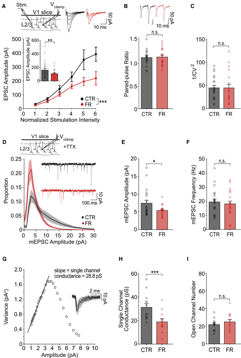
Figureu00a02
Reduced AMPAR currents are mediated by a reduction in single-channel AMPAR conductance in food-restricted mice (A) Top left: schema of voltage-clamp recordings of layer 2/3 neurons in V1 slices. A sti...

Figureu00a03
Reduced AMPAR currents are compensated by an increased input resistance and a depolarized resting membrane potential in food-restricted mice (A) Schema of current-clamp recording of layer 2/3 neurons ...

Figureu00a04
Increased subthreshold variability contributes to broadened orientation tuning in food-restricted mice (A) Sample current-clamp recordings of layer 2/3 neurons in awake mice during presentation of dri...

Figureu00a05
Increased input resistance and depolarization of the resting membrane potential amplifies subthreshold variability, leading to broadened orientation tuning (A) Hodgkin-Huxley type model neuron with re...

Figureu00a06
Food restriction results in a decrease in cortical coding precision and impaired fine visual discrimination (A) Top: example field of view of GCaMP6s-labeled layer 2/3 neurons (scale bar: 10u00a0u03bc...

Figureu00a07
Food restriction affects cortical coding precision via leptin signaling (A) Experimental timeline and animal weight. (B) Mean leptin levels (one-way ANOVA, pu00a0< 0.0001; post hoc Sidaku2019s test...
Figure images are served from the NIH/NLM PubMed Central Open Access Subset or Europe PMC; copyright remains with the publishers and authors.
💬 Discussion
0 commentsNo comments yet. Be the first to start a discussion!
Leave a Comment