Abstract
Undersampling and pixelation affect a number of imaging systems, limiting the resolution of the acquired images, which becomes particularly significant for wide-field microscopy applications. Various super-resolution techniques have been implemented to mitigate this resolution loss by utilizing sub-pixel displacements in the imaging system, achieved, for example, by shifting the illumination source, the sensor array and/or the sample, followed by digital synthesis of a smaller effective pixel by merging these sub-pixel-shifted low-resolution images. Herein, we introduce a new pixel super-resolution method that is based on wavelength scanning and demonstrate that as an alternative to physical shifting/displacements, wavelength diversity can be used to boost the resolution of a wide-field imaging system and significantly increase its space-bandwidth product. We confirmed the effectiveness of this new technique by improving the resolution of lens-free as well as lens-based microscopy systems and developed an iterative algorithm to generate high-resolution reconstructions of a specimen using undersampled diffraction patterns recorded at a few wavelengths covering a narrow spectrum (10-30 nm). When combined with a synthetic-aperture-based diffraction imaging technique, this wavelength-scanning super-resolution approach can achieve a half-pitch resolution of 250 nm, corresponding to a numerical aperture of ~1.0, across a large field of view (>20 mm2). We also demonstrated the effectiveness of this approach by imaging various biological samples, including blood and Papanicolaou smears. Compared with displacement-based super-resolution techniques, wavelength scanning brings uniform resolution improvement in all directions across a sensor array and requires significantly fewer measurements. This technique would broadly benefit wide-field imaging applications that demand larger space-bandwidth products.
🔬 Techniques
💻 Software
✨ Fluorophores
🏭 Microscope Brands
💻 Software Details
🏛️ Research Organizations (ROR)
Affiliated research institutions:
📋 Methods
Optical setup
As depicted in Figure 1 , the optical setup of the lens-free microscope consists of three major components: a light source, an image sensor array, and a specimen. A fiber-coupled, wavelength-tunable light source (WhiteLase-Micro, model VIS, Fianium Ltd, Southampton, UK) is used to perform the wavelength scanning. During the imaging process, the central wavelength of the source is scanned within a spectral range of 10–30 nm (for example, from 498 to 510 nm) with a step size of ~3 nm. The spectral linewidth of illumination at each wavelength is ~2 nm, and the power of the light source is adjusted to ~20 μW. The image sensor chip is a color CMOS sensor chip with a pixel size of 1.12 μm manufactured for cellphone camera modules (IU081, Sony Corporation, Tokyo, Japan). During the imaging process, the specimen is mounted on a transparent substrate and placed 100–500 μm above the image sensor chip. We merged our wavelength-scanning-based pixel super-resolution approach with both multi-height 11 and synthetic aperture imaging 12 configurations to obtain phase-retrieved, high-resolution reconstructions of the specimen. For synthetic-aperture-based imaging 12 , the fiber outlet of the light source is mounted on a rotational arm (PRM1Z8, Thorlabs, Newton, NJ, USA), and the image sensor is placed on a stage that can rotate over a horizontal plane. Therefore, the incident light can be set to arbitrary illumination angles, which is required for the synthetic aperture approach. For multi-height-based phase retrieval 9 , 11 , the incremental height change between the image sensor and the specimen is enabled by a mechanical positioning stage (MAX606, Thorlabs). The image sensor is mounted on this mechanical stage, whereas the specimen is held by a three-dimensional-printed sample holder. After completing image capture for each height, the stage lowers the image sensor by 10–15 μm on average before the image capture for the next height starts. During the imaging process, all the necessary steps, including the wavelength scanning of the light source, multi-height and synthetic-aperture-related scans and data acquisition using the image sensor chip are automated by a custom-written LabVIEW code (Version 2011, National Instruments, Austin, TX, USA). Wavelength calibration and dispersion compensation Wavelength calibration of our light source is achieved using an optical spectrum analyzer (HR2000+, Ocean Optics, Amersham, UK). The intensity-weighted average wavelength of each measured spectrum is considered as our illumination wavelength. To achieve optimal resolution, the refractive index of the glass substrate (100 μm, N-BK7, Schott AG, Mainz, Germany) at each wavelength is also corrected using the dispersion formula for borosilicate glass.
Show full methods section
Optical setup
As depicted in Figure 1 , the optical setup of the lens-free microscope consists of three major components: a light source, an image sensor array, and a specimen. A fiber-coupled, wavelength-tunable light source (WhiteLase-Micro, model VIS, Fianium Ltd, Southampton, UK) is used to perform the wavelength scanning. During the imaging process, the central wavelength of the source is scanned within a spectral range of 10–30 nm (for example, from 498 to 510 nm) with a step size of ~3 nm. The spectral linewidth of illumination at each wavelength is ~2 nm, and the power of the light source is adjusted to ~20 μW. The image sensor chip is a color CMOS sensor chip with a pixel size of 1.12 μm manufactured for cellphone camera modules (IU081, Sony Corporation, Tokyo, Japan). During the imaging process, the specimen is mounted on a transparent substrate and placed 100–500 μm above the image sensor chip. We merged our wavelength-scanning-based pixel super-resolution approach with both multi-height 11 and synthetic aperture imaging 12 configurations to obtain phase-retrieved, high-resolution reconstructions of the specimen. For synthetic-aperture-based imaging 12 , the fiber outlet of the light source is mounted on a rotational arm (PRM1Z8, Thorlabs, Newton, NJ, USA), and the image sensor is placed on a stage that can rotate over a horizontal plane. Therefore, the incident light can be set to arbitrary illumination angles, which is required for the synthetic aperture approach. For multi-height-based phase retrieval 9 , 11 , the incremental height change between the image sensor and the specimen is enabled by a mechanical positioning stage (MAX606, Thorlabs). The image sensor is mounted on this mechanical stage, whereas the specimen is held by a three-dimensional-printed sample holder. After completing image capture for each height, the stage lowers the image sensor by 10–15 μm on average before the image capture for the next height starts. During the imaging process, all the necessary steps, including the wavelength scanning of the light source, multi-height and synthetic-aperture-related scans and data acquisition using the image sensor chip are automated by a custom-written LabVIEW code (Version 2011, National Instruments, Austin, TX, USA). Wavelength calibration and dispersion compensation Wavelength calibration of our light source is achieved using an optical spectrum analyzer (HR2000+, Ocean Optics, Amersham, UK). The intensity-weighted average wavelength of each measured spectrum is considered as our illumination wavelength. To achieve optimal resolution, the refractive index of the glass substrate (100 μm, N-BK7, Schott AG, Mainz, Germany) at each wavelength is also corrected using the dispersion formula for borosilicate glass.
Sample preparation
The grating lines used for resolution quantification are fabricated on a ~100 μm glass slide (N-BK7, Schott AG) using focused ion beam milling. Unstained Papanicolaou (Pap) smear slides are prepared through the ThinPrep method (Hologic, Inc., Marlborough, MA, USA). The blood smear samples are prepared using EDTA (ethylenediaminetetraacetic acid) anticoagulated human blood and stained with Wright’s stain 38 . Mathematical formalism of wavelength-scanning pixel super-resolution We assume that the specimen is a thin object mounted on a plane parallel to the image sensor chip and that the specimen is sequentially illuminated by multiple wavelengths { λ k }. At a given wavelength λ k , the object wave can be written as o k ( x , y )=1+ s k ( x , y ), where s k ( x , y ) represents the scattered object wave, immediately at the exit of the object plane ( z =0, in Figure 1a ). The two-dimensional Fourier transform of o k ( x , y ) can be written as O k ( f x , f y )= δ ( f x , f y )+ S k ( f x , f y ). At the image sensor plane ( z = z 0 in Figure 1a ), the Fourier transform of the intensity distribution, i k ( x , y ), can be written as (see Supplementary Information for details): To simplify our notation, we hide the expression of the variables for spatial frequencies ( f x , f y ), and the superscript ‘−’ represents (− f x , − f y ). On the right-hand side of Equation (1) , the first item, δ , represents the background intensity; the second and third items are conjugate holographic terms, which represent the interference of the scattered object wave with the background wave at the sensor plane. The fourth item is the self-interference term, which can be considered negligible for weakly scattering objects. The expression for T k can be written as follows: Where H k ( f x , f y ) is the free space transfer function, and the frequency shifts f x,k and f y,k are determined by the illumination wavelength and the incident angle (refer to the Supplementary Information for details). After the object intensity is sampled by an image sensor array with a pixel pitch of Δ x and Δ y , the discrete Fourier transform of the sensor’s output can be expressed as follows 39 : where u and v are integers and f x and f y are discrete spatial frequency values. Note that I pix ,k ( f x , f y )= I k ( f x , f y )· P k ( f x , f y ), where P k ( f x , f y ) represents the Fourier transform of the pixel function, that is, the two-dimensional responsivity distribution 40 within each pixel: p k ( x , y ). Variables u and v represent the order of spatial aliasing due to pixelation, and ( u , v )=(0,0) corresponds to the non-aliased real (that is, target) signal. The periodic nature of the discrete Fourier transform enables us to extend the expression of I sampled, k to a broader frequency space by upsampling ( Figure 2 ). Based on these definitions, we can express the undersampled or pixelated lens-free hologram at a given wavelength λ k as follows: The non-aliased target signal o k ( x , y ) or its spatial Fourier spectrum can be obtained under ( u , v )=(0,0), that is, δ 00 + S 00, k , which can be written as follows: On the left side of Equation (5) , we retain the pixel function P 00, k , which can be removed later in the last step of the image reconstruction, using, for example, spatial deconvolution with a Wiener filter 41 , as illustrated in ref. 40 . Equation (5) also shows that to obtain the non-aliased object at ( u , v )=(0,0), one needs to eliminate or subtract four terms from the upsampled and back-propagated holographic term (that is, ). To this end, the first item to eliminate, , is the twin image noise, a characteristic artifact of in-line holography. The second term in Equation (5) , which contains and ( u ≠0, v≠ 0) in the summation, represents the effects of spatial aliasing and undersampling for both the real and twin image terms. The third item, which contains in the summation, is the periodic background artifact generated during the upsampling process, and the last item is the self-interference term and its upsampling related artifacts. Starting with the next sub-section, we will discuss a two-stage reconstruction algorithm for eliminating all four of these items listed on the right side of Equation (5) using wavelength scanning to enable super-resolved reconstructions of complex (that is, phase and amplitude) object functions. Reconstruction Stage 1: generation of a high-resolution initial guess of the specimen using wavelength diversity As depicted in Figure 2 , the reconstruction of the specimen image involves two stages. First, it should be noted that in Equation (5) the functions have complex values with unit amplitude, and their phases are highly sensitive to changes in wavelength (see the Supplementary Information for details). Therefore, when the illumination wavelength ( λ k ) is scanned over K different wavelengths that are uniformly spread across a narrow bandwidth, the set of functions can be considered rotating unit vectors, and by summing all these rotating vectors as a function of wavelength, we obtain the following: This expression indicates that by summing all the back propagations at different wavelengths (for example, over a narrow spectral range of 10–30 nm), the reconstructed image, that is, or , can be significantly enhanced, whereas the spatial aliasing and undersampling-related terms with will be considerably suppressed. Therefore, in this first stage of our reconstruction process, we generate a high-resolution initial guess of the specimen by summing all the upsampled and back-propagated raw measurements, that is, low-resolution diffraction patterns. We subtract the artifact items { δ uv ( u ≠0, v ≠0)} before the back-propagation step to create a cleaner image. It should be noted that modifying Equation (6) into a weighted average at each spatial frequency point could achieve better suppression of spatial aliasing and undersampling-related artifacts. However, using our current computation platform, which is based on a central processing unit, the search for optimal weighting factors at each frequency point will significantly increase the total computation time. Therefore, in this proof-of-concept implementation, we choose a simpler summation approach to minimize the computation time for the generation of the initial object guess. The spatial aliasing and undersampling-related artifacts of this initial guess will be further eliminated and cleaned up during the second stage of our algorithm, as will be detailed next. Reconstruction Stage 2: multi-wavelength-based iterative pixel super-resolution and phase retrieval The second stage of our numerical reconstruction involves an iterative algorithm, which contains four sub-steps in each iteration: (1) Knowing each raw measurement’s corresponding wavelength and incidence angle, we apply the corresponding plane wave illumination on the initial guess of the specimen (from Stage 1, discussed above) and propagate the optical field from the object plane to the image sensor plane using the angular spectrum approach 42 . (2) The amplitude of the high-resolution field on the image sensor plane is updated using the low-resolution measurement at the corresponding wavelength. To this end, the intensity of the high-resolution field is convolved with the image sensor’s pixel function and downsampled to the same grid size as the pixelated raw measurement. The difference between the raw measurement and the downsampled intensity map is considered a low-resolution ‘correction’ map for each illumination wavelength. A high-resolution correction map can then be generated by taking the Kronecker product of this low-resolution map and the pixel function. To perform a smooth update, this high-resolution correction map is added to the high-resolution intensity distribution with a relaxation parameter, typically set to ~0.5 (see the Supplementary Information for details). After the smoothed update, a Wiener deconvolution filter that incorporates the image sensor’s noise level is applied to this updated intensity distribution. The square root of this filtered high-resolution intensity distribution is then applied to the amplitude of the field on the sensor plane while the phase map is kept unaltered. (3) This updated field is then back-propagated to the object plane. (4) The back-propagated field is used to update the transmission field on the object plane. This update is performed in the frequency domain ( Figure 2 ) within a circular area whose center is determined by the corresponding illumination wavelength and angle. The radius of this circle is defined by the boundary within which all the spatial frequencies experience an attenuation of less than 3 dB after propagation in the spatial domain. This update on the object plane is also smoothed using a relaxation factor of ~0.5. After the update, the phase of the field on the object plane is converted to an optical path length map, and its amplitude is directly used as the transmission of the object. The four steps described above are performed for every raw (that is, undersampled) measurement captured by the image sensor array. It is considered one iteration cycle when each one of the raw measurements has been used for amplitude update. Typically after 5–10 iteration cycles, the reconstruction converges. The convergence condition for the iteration is defined as follows 43 : where is the sum-squared error between the raw measurement and the downsampled intensity map 43 , ‘ itr ’ is the iteration number, and ε is a convergence constant determined by the noise level of the raw (that is, undersampled) measurements. Phase retrieval using multi-height and synthetic aperture techniques Multi-height 9 , 11 , 44 , 45 , 46 and synthetic aperture 12 techniques have been proven to be robust phase retrieval methods for lens-free on-chip imaging. In previously reported lens-free reconstructions 9 , 11 , 12 , pixel super-resolution and phase retrieval are carried out sequentially: at each height or illumination angle, lateral shift-based pixel super-resolution is first performed to obtain high-resolution diffraction patterns on the image sensor plane. These super-resolved diffraction patterns are then used by an iterative phase retrieval algorithm, in which wave propagations between the object plane and the image sensor plane are executed repeatedly 9 , 11 , 12 . However, in wavelength-scanning-based pixel super-resolution, raw measurements are essentially undersampled versions of different holograms. Therefore, we choose to use the same iterative algorithm detailed in the previous sub-section (that is, Reconstruction Stage 2) to realize resolution enhancement and phase retrieval altogether. More specifically, in the multi-height configuration, the specimen is illuminated sequentially at each wavelength, and the corresponding lens-free holograms are captured before the vertical scanning stage moves the sample or the image sensor to the next height. Each height will be labeled with index l ; therefore, all the measurements { I sampled , k } and the corresponding transfer functions { H k } and { T uv, k } that are used in the previous derivations can be relabeled as { I sampled , kl }, { H kl } and { T uv, kl }, respectively. During the numerical reconstruction process, all the raw holograms are upsampled, back-propagated, and then summed together to generate the high-resolution initial guess at a given height. In Stage 2 of our reconstruction algorithm, the aforementioned four-step process is applied to each raw measurement. The same set of operations and processing also apply to the synthetic aperture technique 12 , except that index l now refers to each illumination angle instead of sample height. In general, for pathology slides such as blood smears and Pap smears, the optical path length difference between the specimen (that is, biological tissue) and the medium (that is, air or the sealing glue) is rather small. Under these circumstances, phase unwrapping is not a concern; therefore, in the phase recovery process, we can use a scrambled order of { I sampled, kl } in each iteration cycle. However, when working with samples with larger optical path length differences, such as grating lines carved into a glass substrate, one extra step, that is, phase unwrapping, must be added after the reconstruction, and the order of iterations must be modified accordingly, which will be detailed in the next sub-section. Multi-wavelength phase unwrapping A robust phase unwrapping algorithm requires high-resolution and phase-retrieved reconstructions at multiple wavelengths; therefore, we divide the raw measurements into subsets, in which the wavelengths are identical or very similar (for example, Δ λ ≤5 nm), and perform the four-step reconstruction process previously discussed (as part of the Reconstruction Stage 2) on each subset separately. For example, reconstruction number 1 uses subset { I sampled , kl | k =1, l =1,… L }, No. 2 uses { I sampled , kl | k =2, l =1,… L } and so on. When the iterations for all these subsets are completed, we obtain high-resolution (that is, super-resolved) phase-retrieved reconstructions at multiple wavelengths, that is, { O k }, whose phase maps { φ k, wrapped } need unwrapping. Using these wrapped phase maps { φ k, wrapped } at multiple wavelengths, we perform phase unwrapping to accurately reveal the optical path length differences between the specimen and the surrounding medium. Assuming that the optical path length difference is ΔL ( x , y ), the phase distribution at the object plane at each wavelength can be written as φ k ( x , y )=2 π ·Δ L ( x , y )/ λ k . The wrapped phase can thus be expressed as φ k, wrapped ( x , y )= φ k ( x , y )±2 Nπ , where − π < φ k, wrapped ≤ π and N is an integer. These resulting wrapped phase maps { φ k, wrapped } that are generated through super-resolved and phase-retrieved reconstructions at multiple wavelengths are then fed into an optimization algorithm 47 that finds the optimum path length Δ L opt ( x , y ) at each spatial point ( x , y ) by minimizing a cost function defined as follows: To avoid convergence to a local minimum and reduce the computation cost/time, we define a search range of [Δ L 0 −min{ λ k }/2, Δ L 0 +min{ λ k }/2], where Δ L 0 is the initial guess of the optical path length: where the total number of wavelengths ( K ) is typically 5–10. Within this search interval, we scan the values to find the optical path length Δ L opt ( x , y ) that minimizes the cost function, resulting in an unwrapped object phase image. Computation platform used for super-resolved image reconstructions Our reconstructions are performed using MATLAB (Version R2012a, MathWorks, Natick, MA, USA) on a desktop computer equipped with a 3.60-GHz central processing unit (Intel Xeon E5-1620) and 16 GB of random-access memory. For a 1 × 1 mm 2 sub-region with an upsampling factor of seven, one iteration of our wavelength-scanning super-resolution routine takes ~1.2 s. For example, one cycle of our algorithm, which undergoes all the undersampled measurements (for example, seven wavelengths for each angle/height, and 22 angles/heights in total), takes ~3 min. In our proof-of-concept implementation, the iterations did not use either GPU (graphics processing unit) or parallel computing, which could significantly improve our overall computation time 10 . The total image reconstruction time could be further improved by implementing the algorithm in the C language rather than MATLAB.
Supplementary Material Supplementary Information Click here for additional data file.
📊 Figures
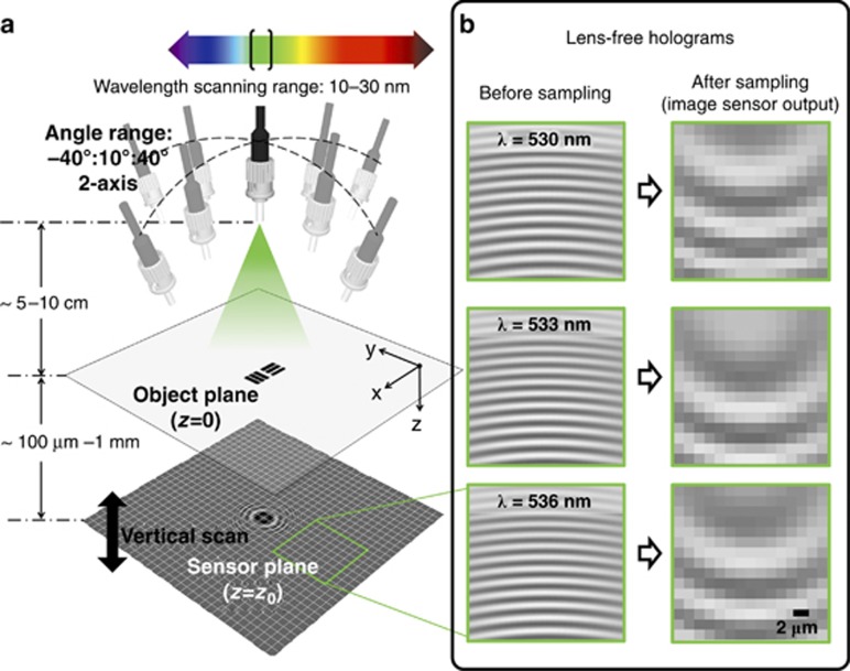
Figure 1
Optical setup of wavelength-scanning pixel-super resolution. ( a ) A lens-free holographic on-chip microscope using wavelength-scanning pixel super-resolution. A fiber-coupled tunable light source is ...
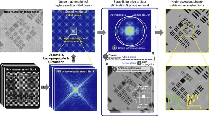
Figure 2
Reconstruction algorithm for wavelength-scanning pixel super-resolution, integrated with multi-height or synthetic-aperture-based lens-free phase retrieval. Refer to the Materials and Methods section ...
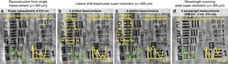
Figure 3
Resolution improvement introduced by wavelength-scanning pixel super-resolution. ( a ) Reconstruction from a single raw measurement captured by an image sensor chip with a pixel pitch of 1.12u2009u03b...
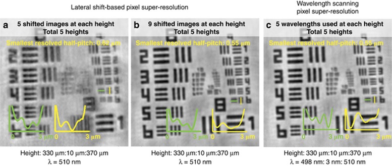
Figure 4
Lens-free imaging using multi-height phase retrieval and wavelength-scanning pixel super-resolution. Five heights are used in each case shown in au2013c . ( a , b ) are lens-free reconstructions using...
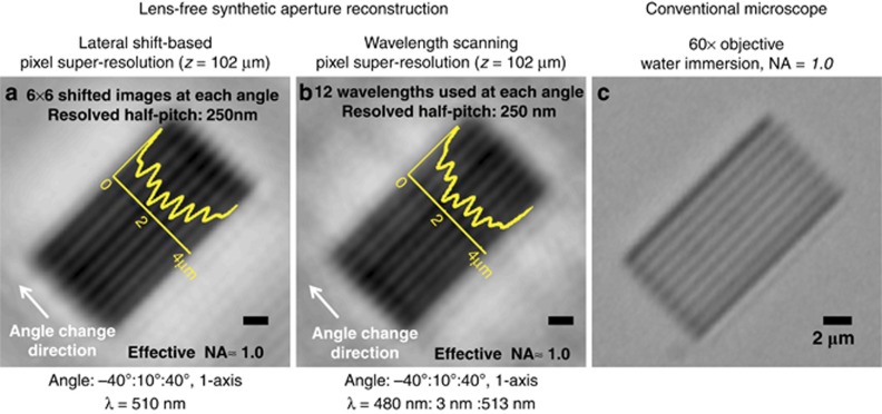
Figure 5
( a ) Lens-free imaging using synthetic aperture and lateral shift-based pixel super-resolution. At each illumination angle, 6 u00d7 6=36 sub-pixel lateral shifts, which are spread evenly over the pix...
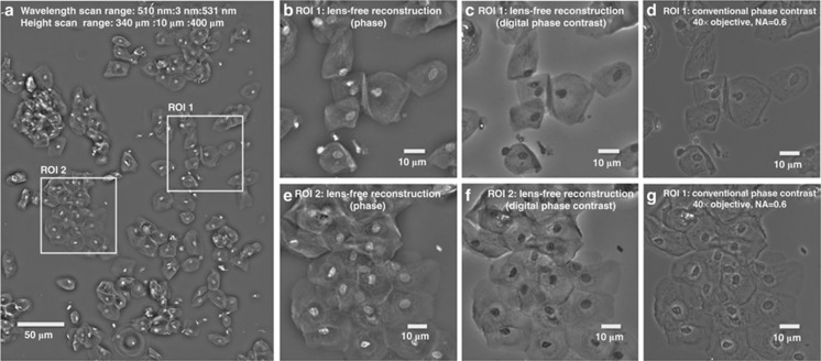
Figure 6
Lens-free imaging of a Papanicolaou (Pap) smear using wavelength-scanning pixel super resolution and multi-height phase retrieval. ( a ) Super-resolved lens-free phase image of the Pap smear. Waveleng...
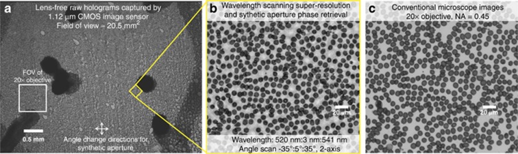
Figure 7
Lens-free imaging of a blood smear using wavelength-scanning pixel super-resolution and synthetic aperture phase retrieval. Wavelength-scanning range: 520u2013541u2009nm, scanning step: 3u2009nm. Angl...
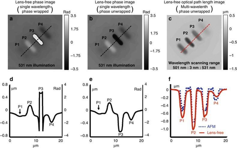
Figure 8
Phase unwrapping using multiple wavelengths. The sample consists of four grating lines carved into a glass substrate using focused ion beam milling. ( a ) Lens-free phase image obtained using a single...
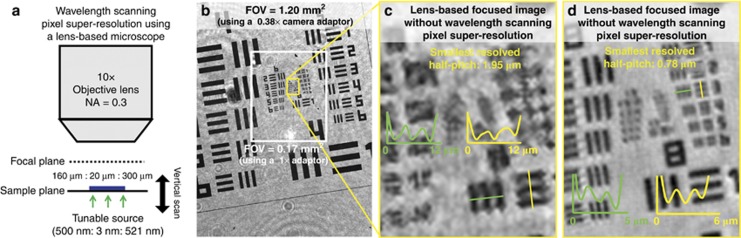
Figure 9
Implementation of wavelength-scanning pixel super-resolution using a lens-based microscope. ( a ) Schematic of the optical setup. In this proof-of-concept experiment, a 10 u00d7 objective lens (NA=0.3...
Figure images are served from the NIH/NLM PubMed Central Open Access Subset or Europe PMC; copyright remains with the publishers and authors.
💬 Discussion
0 commentsNo comments yet. Be the first to start a discussion!
Leave a Comment