Abstract
The primary visual cortex is an excellent model system for investigating how neuronal populations encode information, because of well-documented relationships between stimulus characteristics and neuronal activation patterns. We used two-photon calcium imaging data to relate the performance of different methods for studying population coding (population vectors, template matching, and Bayesian decoding algorithms) to their underlying assumptions. We show that the variability of neuronal responses may hamper the decoding of population activity, and that a normalization to correct for this variability may be of critical importance for correct decoding of population activity. Second, by comparing noise correlations and stimulus tuning we find that these properties have dissociated anatomical correlates, even though noise correlations have been previously hypothesized to reflect common synaptic input. We hypothesize that noise correlations arise from large non-specific increases in spiking activity acting on many weak synapses simultaneously, while neuronal stimulus response properties are dependent on more reliable connections. Finally, this paper provides practical guidelines for further research on population coding and shows that population coding cannot be approximated by a simple summation of inputs, but is heavily influenced by factors such as input reliability and noise correlation structure.
🔬 Techniques
🔭 Microscopes
✨ Fluorophores
🧪 Sample Preparation
🔬 Cell Lines
🏭 Microscope Brands
💻 Software Details
🏛️ Research Organizations (ROR)
Affiliated research institutions:
📋 Methods
Animal preparation
All experimental procedures were conducted with approval of the animal ethics committee of the University of Amsterdam and are largely similar to those described in more detail in Goltstein et al. ( 2013 ). In short, 6 adult male C57BL/6 mice (Harlan) were implanted with a titanium head bar prior to the imaging experiment and were allowed to recover for a minimum of 3 days. On the day of the two-photon calcium imaging experiment, buprenorphine (0.05 mg/kg) was injected subcutaneously 30–60 min before induction of anesthesia with isoflurane (3.0% in 100% oxygen).
Intrinsic signal imaging
(ISI) was performed to localize the primary visual cortex (V1) while the animal was anesthetized lightly (0.8% isoflurane). We subsequently performed a small (2 mm) craniotomy above the retinotopic area responding to visual stimulation with drifting gratings. After the craniotomy, the dura was kept wet with an artificial cerebrospinal fluid (ACSF: NaCl 125 mM, KCl 5.0 mM, MgSO 4 * 7 H 2 O 2.0 mM, NaH 2 PO 4 2.0 mM, CaCl 2 * 2 H 2 O 2.5 mM, glucose 10 mM) buffered with HEPES (10 mM, adjusted to pH 7.4) (Svoboda et al., 1999 ). After removal of the skull, multi-cell bolus loading with Oregon Green BAPTA-1 AM (OGB) and Sulforhodamine 101 (SR101) was performed 230–270 microns below the dura as previously described (Stosiek et al., 2003 ; Goltstein et al., 2013 ). After injection of the dyes, the exposed dura was covered with agarose (1.5% in ACSF) and sealed with a circular cover glass that was fixed to the skull using cyanoacrylate glue. Apparatus and stimulus presentations Dual-channel two-photon imaging recordings (filtered at 500–550 nm for OGB and 565–605 nm for SR101; see Figure 1A ) with a 512 × 512 pixel frame size were performed at a sampling frequency of 25.4 Hz. We used an in vivo two-photon laser scanning microscopy setup (modified Leica SP5 confocal system) with a Spectra-Physics Mai-Tai HP laser set at a wavelength of 810 nm to simultaneously excite OGB and SR101 molecules, as previously described (Goltstein et al., 2013 ). Mice ( n = 6) were kept lightly anesthetized (0.8% isoflurane) during the entirety of the two-photon calcium imaging recordings ( n = 6, 1 data set/animal), while they were presented with 10 repetitions of 8 different directions of square-wave drifting gratings ( n = 80 trials/recording). Visual stimulation duration was 3 s and was alternated by a 5 s blank inter-trial interval during which an isoluminant gray screen was presented. Visual drifting gratings (diameter 60 retinal degrees, spatial frequency 0.05 cycles/degree, temporal frequency 1 Hz) were presented within a circular cosine-ramped window to avoid edge effects at the border of the circular window. All visual stimulation was performed on a 15 inch TFT screen with a refresh rate of 60 Hz positioned at 16 cm from the mouse's eye, which was controlled by MATLAB using the PsychToolbox extension (Brainard, 1997 ; Pelli, 1997 ). A field-programmable gate array (FPGA, OpalKelly XEM3001) was connected to the microscope setup and interfaced with the stimulus computer to synchronize the timing of the visual stimulation with the microscope frame acquisition. Figure 1 (A) Contrast-enhanced average of all x-y movement-corrected frames recorded from an anesthetized mouse during a two-photon calcium imaging experiment used for decoding. The data were obtained by recording fluorescence levels in neurons stained with Oregon Green BAPTA-1 AM (OGB-1 AM). Dual dye-loading with Sulforhodamine-101 (SR-101) was performed to differentiate astrocytes (yellow/orange) from neuronal cell bodies (green). The location marked in blue in the upper part of the example recording is the cell body of the neuron whose stimulus-selective responses are shown in (B) . (B) Activity trace of an example neuron measured by the dF/F 0 (fraction change in fluorescence level relative to a 30 s baseline, which correlates approximately linearly with spiking activity). This neuron responds strongly to gratings moving to the upper left (315°) and lower right (135°), but not to any other moving direction. It is therefore strongly orientation-tuned, but weakly direction-tuned. Each gray line depicts a single trial (−3 to +5 s of stimulus onset) and the mean response per stimulus direction over all ten repetitions is shown in blue. The area shaded in gray shows stimulus presentation time. Depicted in the center graph is the maximum value of the mean response of the neuron per stimulus direction in dF/F 0 . Data preprocessing After a recording was completed small x-y drifts were corrected with an image registration algorithm (Guizar-Sicairos et al., 2008 ) and the recording was manually checked for movement artifacts along the z-axis. If z-drifts occurred during a recording, it was rejected and no further analyses were performed. Regions of interest (neurons, astrocytes, and blood vessels) were determined semi-automatically using custom-made MATLAB software and subsequently dF/F 0 values for all neurons were calculated as previously described (Goltstein et al., 2013 ). In short, for each image frame i a single dF/F 0 value was obtained for each neuron by calculating the baseline fluorescence ( F 0 i ), taken as the mean of the lowest 50% during a 30-s window preceding image frame i . dF is defined as the difference between the fluorescence for that neuron in the given frame and the sliding baseline fluorescence ( d F i = F i −F 0 i ) (Goltstein et al., 2013 ). The mean number of simultaneously recorded neurons/session was 118 (range: 95–144). Neuronal responses to visual stimuli A neuron's response to a certain stimulus was defined as the mean dF/F 0 value of all frames recorded during that single trial's stimulus presentation (see Figure 1B for an example neuron). Stimulus presentation lasted 3.0 s (77 frames) and a single stimulus presentation yields a single response value R , equal to the mean dF/F 0 over all 77 stimulus frames. To obtain a measure of a neuron's orientation selectivity, we calculated the orientation selectivity index (OSI) as (1-circular variance), as previously described by Ringach et al. ( 2002 ). To further parameterize neuronal orientation tuning, we also calculated each neuron's preferred direction by fitting a double von Mises distribution to the neuron's responses, where the peaks of both von Mises functions are opposite to each other (separated by 180°): (1) f ( x | θ , κ 1 , κ 2 , μ 0 ) = e κ 1 cos ( x − θ ) 2 π I 0 ( κ 1 ) + e κ 2 cos ( x + π − θ ) 2 π I 0 ( κ 2 ) + μ 0 Here, I 0 (κ) is the modified Bessel function of order 0 and x represents the stimulus angle. As can be seen in the equation, we defined the free parameters as θ (preferred direction), κ 1 (concentration parameter at θ), κ 2 (concentration parameter at θ +π) and μ 0 (baseline response). A neuron's preferred direction was defined as the angle with the highest concentration parameter (which could be either κ 1 or κ 2 ). Signal correlations In many cases neuronal responses in V1 to drifting gratings can be fairly accurately approximated by circular von Mises distributions. However, in order to more fully capture similarities and differences between the responses that neurons show to drifting gratings of different directions, we calculated signal correlations between all neuronal pairs in each recording. We defined each direction as a separate stimulus type and calculated a neuron's mean response vector R , where the elements of R are the neuron's mean responses to each direction θ ( R θ ): (2) R ¯ = [ R ¯ 0 , R ¯ 45 … R ¯ 315 ] We then calculated the pairwise signal correlation as the Pearson correlation between two neurons' ( i , j ) response vectors: (3) ρ i , j signal = corr ( R ¯ i , R ¯ j ) Since the decoding algorithms used to extract information from the population response depend on the difference in response between neurons for different stimulus directions, high signal correlations between two neurons indicate that there is a large redundancy in information that these neurons provide to the decoder. Noise correlations Complementary to signal correlations, which provide an index of the similarity between pairs of neurons in their mean response to the different stimulus types, are noise correlations, which give an indication of the similarity in trial-by-trial response variability between neurons. We first calculated a response vector for each stimulus type θ, where each element in the vector is the neuron's response to a single presentation i of that stimulus direction: (4) R θ = [ R θ i … R θ n ] , where n is ten, since we have ten repetitions per direction. Because we aim to compare a single noise correlation value per neuronal pair, we took the mean noise correlation over all eight stimulus directions θ = 0°–315° (with steps of 45°): (5) ρ i , j noise = ∑ θ = 0 315 corr ( R i , θ , R j , θ ) 8 The noise correlation is therefore an index of the mean shared trial-by-trial variability over all stimulus directions. Decoding sample bootstrapping All decoding algorithms (described in detail in the following paragraphs) were tested on their ability to recover the presented stimulus direction from the neuronal population activity during single trials. To quantify their dependence on the number of neurons included, we took random subsamples of neurons (100 iterations) from each data set (ranging from 95 to 144 neurons simultaneously recorded neurons) for all tested sample sizes (1–90 neurons, each neuron was included only once). For each random sample we trained the decoder on the activity of the randomly included neurons for all 80 trials (8 directions, 10 repetitions) and subsequently decoded the presented direction of each trial from the population activity of only these neurons. Since the smallest data set consisted of 95 neurons, we ran our resampling procedures up to a maximum population size of 90 neurons. We performed these resamplings independently for each decoding algorithm. Population vector decoding To decode the presented stimulus direction during a given trial, we used the population vector method (Georgopoulos et al., 1986 ) as follows. For each trial, the activity of each neuron was represented as a vector, where the angle (θ) represents the neuron's preferred direction and the magnitude (ρ) corresponds to its activity level ( dF/F 0 ). A resultant population vector can then be calculated by taking the circular mean over all neurons. When the resultant angle was within 22.5 degrees of the actual stimulus direction, it was counted as a “correct” decoding, in all other cases it was marked as “incorrect.” After decoding all trials, the percentage correct decoded was then calculated over all trials, so it could be plotted as in Figure 4 .
Show full methods section
Animal preparation
All experimental procedures were conducted with approval of the animal ethics committee of the University of Amsterdam and are largely similar to those described in more detail in Goltstein et al. ( 2013 ). In short, 6 adult male C57BL/6 mice (Harlan) were implanted with a titanium head bar prior to the imaging experiment and were allowed to recover for a minimum of 3 days. On the day of the two-photon calcium imaging experiment, buprenorphine (0.05 mg/kg) was injected subcutaneously 30–60 min before induction of anesthesia with isoflurane (3.0% in 100% oxygen).
Intrinsic signal imaging
(ISI) was performed to localize the primary visual cortex (V1) while the animal was anesthetized lightly (0.8% isoflurane). We subsequently performed a small (2 mm) craniotomy above the retinotopic area responding to visual stimulation with drifting gratings. After the craniotomy, the dura was kept wet with an artificial cerebrospinal fluid (ACSF: NaCl 125 mM, KCl 5.0 mM, MgSO 4 * 7 H 2 O 2.0 mM, NaH 2 PO 4 2.0 mM, CaCl 2 * 2 H 2 O 2.5 mM, glucose 10 mM) buffered with HEPES (10 mM, adjusted to pH 7.4) (Svoboda et al., 1999 ). After removal of the skull, multi-cell bolus loading with Oregon Green BAPTA-1 AM (OGB) and Sulforhodamine 101 (SR101) was performed 230–270 microns below the dura as previously described (Stosiek et al., 2003 ; Goltstein et al., 2013 ). After injection of the dyes, the exposed dura was covered with agarose (1.5% in ACSF) and sealed with a circular cover glass that was fixed to the skull using cyanoacrylate glue. Apparatus and stimulus presentations Dual-channel two-photon imaging recordings (filtered at 500–550 nm for OGB and 565–605 nm for SR101; see Figure 1A ) with a 512 × 512 pixel frame size were performed at a sampling frequency of 25.4 Hz. We used an in vivo two-photon laser scanning microscopy setup (modified Leica SP5 confocal system) with a Spectra-Physics Mai-Tai HP laser set at a wavelength of 810 nm to simultaneously excite OGB and SR101 molecules, as previously described (Goltstein et al., 2013 ). Mice ( n = 6) were kept lightly anesthetized (0.8% isoflurane) during the entirety of the two-photon calcium imaging recordings ( n = 6, 1 data set/animal), while they were presented with 10 repetitions of 8 different directions of square-wave drifting gratings ( n = 80 trials/recording). Visual stimulation duration was 3 s and was alternated by a 5 s blank inter-trial interval during which an isoluminant gray screen was presented. Visual drifting gratings (diameter 60 retinal degrees, spatial frequency 0.05 cycles/degree, temporal frequency 1 Hz) were presented within a circular cosine-ramped window to avoid edge effects at the border of the circular window. All visual stimulation was performed on a 15 inch TFT screen with a refresh rate of 60 Hz positioned at 16 cm from the mouse's eye, which was controlled by MATLAB using the PsychToolbox extension (Brainard, 1997 ; Pelli, 1997 ). A field-programmable gate array (FPGA, OpalKelly XEM3001) was connected to the microscope setup and interfaced with the stimulus computer to synchronize the timing of the visual stimulation with the microscope frame acquisition. Figure 1 (A) Contrast-enhanced average of all x-y movement-corrected frames recorded from an anesthetized mouse during a two-photon calcium imaging experiment used for decoding. The data were obtained by recording fluorescence levels in neurons stained with Oregon Green BAPTA-1 AM (OGB-1 AM). Dual dye-loading with Sulforhodamine-101 (SR-101) was performed to differentiate astrocytes (yellow/orange) from neuronal cell bodies (green). The location marked in blue in the upper part of the example recording is the cell body of the neuron whose stimulus-selective responses are shown in (B) . (B) Activity trace of an example neuron measured by the dF/F 0 (fraction change in fluorescence level relative to a 30 s baseline, which correlates approximately linearly with spiking activity). This neuron responds strongly to gratings moving to the upper left (315°) and lower right (135°), but not to any other moving direction. It is therefore strongly orientation-tuned, but weakly direction-tuned. Each gray line depicts a single trial (−3 to +5 s of stimulus onset) and the mean response per stimulus direction over all ten repetitions is shown in blue. The area shaded in gray shows stimulus presentation time. Depicted in the center graph is the maximum value of the mean response of the neuron per stimulus direction in dF/F 0 . Data preprocessing After a recording was completed small x-y drifts were corrected with an image registration algorithm (Guizar-Sicairos et al., 2008 ) and the recording was manually checked for movement artifacts along the z-axis. If z-drifts occurred during a recording, it was rejected and no further analyses were performed. Regions of interest (neurons, astrocytes, and blood vessels) were determined semi-automatically using custom-made MATLAB software and subsequently dF/F 0 values for all neurons were calculated as previously described (Goltstein et al., 2013 ). In short, for each image frame i a single dF/F 0 value was obtained for each neuron by calculating the baseline fluorescence ( F 0 i ), taken as the mean of the lowest 50% during a 30-s window preceding image frame i . dF is defined as the difference between the fluorescence for that neuron in the given frame and the sliding baseline fluorescence ( d F i = F i −F 0 i ) (Goltstein et al., 2013 ). The mean number of simultaneously recorded neurons/session was 118 (range: 95–144). Neuronal responses to visual stimuli A neuron's response to a certain stimulus was defined as the mean dF/F 0 value of all frames recorded during that single trial's stimulus presentation (see Figure 1B for an example neuron). Stimulus presentation lasted 3.0 s (77 frames) and a single stimulus presentation yields a single response value R , equal to the mean dF/F 0 over all 77 stimulus frames. To obtain a measure of a neuron's orientation selectivity, we calculated the orientation selectivity index (OSI) as (1-circular variance), as previously described by Ringach et al. ( 2002 ). To further parameterize neuronal orientation tuning, we also calculated each neuron's preferred direction by fitting a double von Mises distribution to the neuron's responses, where the peaks of both von Mises functions are opposite to each other (separated by 180°): (1) f ( x | θ , κ 1 , κ 2 , μ 0 ) = e κ 1 cos ( x − θ ) 2 π I 0 ( κ 1 ) + e κ 2 cos ( x + π − θ ) 2 π I 0 ( κ 2 ) + μ 0 Here, I 0 (κ) is the modified Bessel function of order 0 and x represents the stimulus angle. As can be seen in the equation, we defined the free parameters as θ (preferred direction), κ 1 (concentration parameter at θ), κ 2 (concentration parameter at θ +π) and μ 0 (baseline response). A neuron's preferred direction was defined as the angle with the highest concentration parameter (which could be either κ 1 or κ 2 ). Signal correlations In many cases neuronal responses in V1 to drifting gratings can be fairly accurately approximated by circular von Mises distributions. However, in order to more fully capture similarities and differences between the responses that neurons show to drifting gratings of different directions, we calculated signal correlations between all neuronal pairs in each recording. We defined each direction as a separate stimulus type and calculated a neuron's mean response vector R , where the elements of R are the neuron's mean responses to each direction θ ( R θ ): (2) R ¯ = [ R ¯ 0 , R ¯ 45 … R ¯ 315 ] We then calculated the pairwise signal correlation as the Pearson correlation between two neurons' ( i , j ) response vectors: (3) ρ i , j signal = corr ( R ¯ i , R ¯ j ) Since the decoding algorithms used to extract information from the population response depend on the difference in response between neurons for different stimulus directions, high signal correlations between two neurons indicate that there is a large redundancy in information that these neurons provide to the decoder. Noise correlations Complementary to signal correlations, which provide an index of the similarity between pairs of neurons in their mean response to the different stimulus types, are noise correlations, which give an indication of the similarity in trial-by-trial response variability between neurons. We first calculated a response vector for each stimulus type θ, where each element in the vector is the neuron's response to a single presentation i of that stimulus direction: (4) R θ = [ R θ i … R θ n ] , where n is ten, since we have ten repetitions per direction. Because we aim to compare a single noise correlation value per neuronal pair, we took the mean noise correlation over all eight stimulus directions θ = 0°–315° (with steps of 45°): (5) ρ i , j noise = ∑ θ = 0 315 corr ( R i , θ , R j , θ ) 8 The noise correlation is therefore an index of the mean shared trial-by-trial variability over all stimulus directions. Decoding sample bootstrapping All decoding algorithms (described in detail in the following paragraphs) were tested on their ability to recover the presented stimulus direction from the neuronal population activity during single trials. To quantify their dependence on the number of neurons included, we took random subsamples of neurons (100 iterations) from each data set (ranging from 95 to 144 neurons simultaneously recorded neurons) for all tested sample sizes (1–90 neurons, each neuron was included only once). For each random sample we trained the decoder on the activity of the randomly included neurons for all 80 trials (8 directions, 10 repetitions) and subsequently decoded the presented direction of each trial from the population activity of only these neurons. Since the smallest data set consisted of 95 neurons, we ran our resampling procedures up to a maximum population size of 90 neurons. We performed these resamplings independently for each decoding algorithm. Population vector decoding To decode the presented stimulus direction during a given trial, we used the population vector method (Georgopoulos et al., 1986 ) as follows. For each trial, the activity of each neuron was represented as a vector, where the angle (θ) represents the neuron's preferred direction and the magnitude (ρ) corresponds to its activity level ( dF/F 0 ). A resultant population vector can then be calculated by taking the circular mean over all neurons. When the resultant angle was within 22.5 degrees of the actual stimulus direction, it was counted as a “correct” decoding, in all other cases it was marked as “incorrect.” After decoding all trials, the percentage correct decoded was then calculated over all trials, so it could be plotted as in Figure 4 .
Template matching algorithm
One step up in complexity from the population vector is the template matching algorithm (Lehky and Sejnowski, 1990 ; Zhang et al., 1998 ; van Duuren et al., 2008 , 2009 ). While in the population vector method each neuron is represented only by a preferred direction and its activity level, template matching compares the population activity to response templates of different stimulus types. These templates are generated by taking the mean activity across trials during the presentation of each stimulus direction (θ) for each neuron, resulting in a “template population activity.” The similarity of this template ( R θ ) to the actual population activity ( R stim ) is given by (6) Θ θ = ∑ i = 1 N R i stim · R i θ ‖ R θ ‖ · ‖ R stim ′ ‖ , where i indexes the N elements (neurons) of R , and · indicates multiplication. The similarity index Θ is calculated for all eight directions and the decoded output is determined by taking the direction with the highest similarity to the population activity. The non-scale sensitive fano factor (rFano) The Fano factor provides an indication of the variability of neuronal responses. Two-photon calcium imaging yields neuronal responses that are given as dF/F 0 , where the relationship between the actual spiking rate and the dF/F 0 is approximately linear per neuron, but varies over neurons (Kerr et al., 2005 ; Greenberg et al., 2008 ). Compared to firing rates, neuronal dF/F 0 responses are therefore scaled by an arbitrary constant c by which both the mean (μ) and standard deviation (σ) of its responses over the entire recording are multiplied. The scaling sensitivity is described by the following equation: (7) Fano = σ 2 · c 2 μ · c Therefore, Fano factors calculated from calcium imaging data are only accurate when c = 1, as scaling (of the firing rate) has a disproportionally larger effect on the variance than the mean. For this reason, raw Fano Factors from calcium imaging cannot be simply translated to the Fano Factors of the raw firing rates. To correctly calculate the variability of calcium transient data, the variance and mean activity level per neuron must be normalized, thereby removing the constant c from the equation. While it is not possible to compute the raw Fano factors of the unknown firing rates, it is possible, however, to compute a Fano factor based on relative changes in mean and variance across stimulus dimensions. We therefore define the ratio Fano factor (r Fano ) as follows: (8) r Fano = σ p 2 / σ n p 2 μ p / μ n p where μ p and σ 2 p are the mean response and variance over trials to the neuron's preferred (P°) and opposite (P° + 180°) direction, and μ np and σ 2 np are the mean response and variance to the other six moving directions. This way, the mean and variance are described as fractional increases in activity and variability from non-preferred stimulus epochs to preferred stimulus epochs. Because c 2 appears in both variance terms and c appears in both mean response terms, the r Fano factor is no longer scale sensitive. Normalized template matching In an attempt to improve the performance of the template matching algorithm, we performed a similar decoding operation, but now on the z-scored rather than the raw dF/F 0 activity values. The new equation becomes (9) Θ θ = ∑ i = 1 N Z i stim · Z i θ ‖ Z θ ‖ · ‖ Z stim , ‖ , where Z is an index that describes a neuron's dF/F 0 response ( R ) for any time point ( i ) as the number of standard deviations (σ) from the mean dF/F 0 calculated over the entire recording ( R all ): (10) Z i = ( R i − R ¯ all ) σ R all Therefore a neuron that shows a high mean activation level ( R all ), but an even higher variability σ R all (high Fano factor) will contribute less to the template similarity than a neuron with a low activation level and an even lower variability (low Fano factor). Bayesian maximum-likelihood (ML) The final algorithm we used was a Bayesian decoder. Bayes' rule is given by (11) P ( θ | A pop ) = P ( A pop | θ ) P ( θ ) P ( A pop ) , where P(θ), the prior, is the prior probability of having direction θ; P(θ | A pop ), the posterior, is the probability of this trial's population activity being caused by direction θ; P( A pop | θ), the likelihood, represents the probability that stimulus direction θ will result in pattern A pop ; and P( A pop ) is the probability of activation pattern A pop , or model evidence—a normalization term. It has been shown before that there is little difference in performance between uniform and natural priors—at least for retinal ganglion cells (Jacobs et al., 2009 )—so for the following results we assumed a uniform prior [P(θ) is equal for all directions] to simplify computational procedures. Note that P( A pop ) is identical for all stimulus directions, since the term θ is not present. Therefore, for a given direction θ, the posterior probability is proportional to the likelihood. The likelihood distribution for a certain direction, say θ = 90 degrees, for any neuron i was given by a Gaussian approximation based on the mean (μ) and standard deviation (σ) of its response to stimuli with that direction during training trials (Figure 2 ); in our case, we included all 80 trials to determine the likelihood distributions. Note that these Gaussians are not tuning curves, but rather an approximation of the dF/F 0 response distribution for a single stimulus direction. The posterior probability for that direction can then be extracted by taking the value of the Gaussian likelihood distribution at the given neuronal activation level A . The population posterior probability distribution for that direction can be calculated by taking the product over the posterior probabilities for all n neurons: (12) P ( θ | A pop ) ∝ ∏ i = 1 n P ( θ | A ) i Figure 2 Graphical representation of the Bayesian decoding scheme shows the process for one example neuron i for a single stimulus direction (90°) in one test trial . The probability of responses to a 90° stimulus [P(A i | θ = 90°)] for this neuron is approximated by a Gaussian distribution (blue curve) with a mean (μ i , gray) and standard deviation (σ i , black) equal to those estimated from training trials where this stimulus direction was presented. For this example to-be-decoded test trial, the neuron's activation level (A i , red) was close to the neuron's mean response to stimuli with a direction of 90 degrees; therefore the posterior probability [P(θ = 90° | A i ), green] that the stimulus was 90 degrees is relatively high based on only this neuron's activation level and tuning. This procedure is repeated for all stimulus directions and the posterior probabilities for all neurons are multiplied. The stimulus direction with the highest probability is subsequently chosen as the maximum-likelihood (ML) read out. Now the decoded direction can be read out by taking the direction with the highest probability.
Jackknifing procedure
One question that can be addressed with these decoding algorithms is whether certain properties of a neuronal response correlate with decoding performance. We therefore performed a bootstrapping procedure (1000 iterations) per recording to select random groups of neurons (ranging in size from 2 to 15) from the whole datasets of 95–144 neurons. Each bootstrap resampling was followed by a jackknife procedure applied to all neurons in the randomly selected group to quantify the contribution of these single neurons to the decoding algorithm's performance. A jackknifing procedure provides insight into the contribution of a single neuron within a sample by taking away that neuron from the rest of the sample and comparing the properties (i.e., decoding performance) of the sample with and without this neuron. This procedure can be repeated for each neuron in the sample and yields a change in decoding performance per neuron that can be compared to other properties of the neuron. For example, jackknifing a certain neuron from a sample that has a high OSI might result in a different change in decoding performance than jackknifing a different neuron from the same sample having a low OSI. This way, the impact of several neuronal properties on decoding performance can be assessed. We normalized the decoding improvement effected by the jackknifed neuron for the number of neurons in the sample by defining the decoding improvement index D i as (13) D i = N D − ( N − 1 ) D ¬ i where N is the sample size, D the decoding accuracy of the algorithm using the entire cluster and D ¬ i is the accuracy using the entire cluster except the jackknifed neuron ( i ). The decoding improvement was then binned and averaged over all points per bin from all 6 data sets (see Figure 6 ). Tuning property interdependency Three important factors that may influence how much information on stimulus direction a neuron contributes to a neuronal cluster are the neuron's preferred orientation (PO), its signal correlation (SC) and its noise correlation (NC) with other members of the cluster. To further quantify if and how these properties show interdependencies, and vary with intersomatic distance (ID) in the imaging plane, we performed a pairwise comparison between neurons for these properties. For all neuronal pairs in all sessions we computed the SC, NC, ID and angular difference in preferred orientation (dPO). We then pooled data points from all sessions and performed a regression analysis to test if there were significant correlations between ID-SC, ID-NC, ID-dPO, SC-NC, SC-dPO and NC-dPO. Two properties were judged to be significantly interdependent when the 99% confidence interval for the regression slope did not overlap with 0. To determine the significance of a difference in slopes between dependent properties for a given independent property (either ID or SC), we z-scored the values of the dependent variable and performed another set of linear regressions. Because of this normalization, we could now quantitatively compare the relative slopes between ID-SC, ID-NC and ID-dPO, and between SC-NC and SC-dPO by assessing whether the 99% confidence intervals of these regression slopes overlapped. Removing biases in tuning property interdependency As will be further elaborated in the Results section, it is possible that the previously described analysis shows significant relationships between neuronal properties that depend on mean differences in those properties between data sets, when in fact these properties are not significantly related within data sets. To control for such possible biases due to across-recording differences, we pooled all neuronal pairs into data bins for ID (0 to 200 with steps of 40 microns), SC (−0.7 to +0.7 with steps of 0.2) and NC (−0.175 to +0.275 with steps of 0.05). These bins were chosen so that at least 90% of all neuronal pairs per data set would be included in the analysis, with the number of points per bin still sufficiently large for robust data analysis. We then computed the minimal number of pairs for each bin for each calcium imaging data set and used this number as the resample size for a bootstrapping procedure (256, 305, and 84 pairs/bin/recording for ID, SC, and NC respectively). For each bootstrapping iteration ( n = 1000), all bins received this number of randomly selected data points (neuronal pairs) from each data set, so that no across-recording differences in mean neuronal property values could lead to biases in the pooled resampled data set. We then performed a linear regression on each randomly sampled set and computed the 99% confidence intervals of the regression slopes to determine whether there was a significant correlation between two neuronal properties.
Jackknifing procedure
One question that can be addressed with these decoding algorithms is whether certain properties of a neuronal response correlate with decoding performance. We therefore performed a bootstrapping procedure (1000 iterations) per recording to select random groups of neurons (ranging in size from 2 to 15) from the whole datasets of 95–144 neurons. Each bootstrap resampling was followed by a jackknife procedure applied to all neurons in the randomly selected group to quantify the contribution of these single neurons to the decoding algorithm's performance. A jackknifing procedure provides insight into the contribution of a single neuron within a sample by taking away that neuron from the rest of the sample and comparing the properties (i.e., decoding performance) of the sample with and without this neuron. This procedure can be repeated for each neuron in the sample and yields a change in decoding performance per neuron that can be compared to other properties of the neuron. For example, jackknifing a certain neuron from a sample that has a high OSI might result in a different change in decoding performance than jackknifing a different neuron from the same sample having a low OSI. This way, the impact of several neuronal properties on decoding performance can be assessed. We normalized the decoding improvement effected by the jackknifed neuron for the number of neurons in the sample by defining the decoding improvement index D i as (13) D i = N D − ( N − 1 ) D ¬ i where N is the sample size, D the decoding accuracy of the algorithm using the entire cluster and D ¬ i is the accuracy using the entire cluster except the jackknifed neuron ( i ). The decoding improvement was then binned and averaged over all points per bin from all 6 data sets (see Figure 6 ).
Explaining the weak performance of the population vector method
The population vector exhibits the weakest performance of the tested algorithms, because it relies on two important assumptions that are violated. First, the population vector method assumes a uniform distribution of preferred directions over the encoded dimension. Clearly, decoding a stimulus direction with a sample size of one neuron will not yield a uniform distribution of preferred directions. This results in a decoded direction that is biased to the direction that is overrepresented by random resampling from the entire population. Moreover, neurons' preferred directions are not uniformly distributed in the visual cortex, but have a bias toward overrepresentation of cardinal directions (Kreile et al., 2011 ). The second violated assumption is that each neuron has a single preferred direction. In V1 most neurons are selective for an axis of orientation (e.g., responding to both upward moving and downward moving) rather than one specific direction (e.g., responding to only upward moving), resulting in a tuning curve with two peaks rather than one (see Figure 3 for an example trial). When the stimulus-driven population activity is divided in two peaks that are separated by 180 degrees, taking a circular mean over the whole population will reduce the size of the signal that is extracted. This reduction takes place because two vectors with opposite directions will result in an average vector that has a magnitude equal to the magnitude in the preferred direction minus the magnitude in the opposite direction. When the population responses in the preferred and opposite direction have similar strengths, the resultant vector has a small magnitude and the decoded direction is especially prone to random imbalances in activation (noise). In essence, the bimodal nature of orientation tuning curves leads to a large decrease in signal-to-noise ratio (SNR) when decoding directions with a population vector. Therefore, although population vector decoding of orientations (Vogels, 1990 ) and of directions with only direction-selective and no orientation-selective neurons work well (Seung and Sompolinsky, 1993 ), direction decoding based on all (mixed) neurons shows very low accuracy. Since fixing or avoiding these two violations would require significant alteration of the population vector algorithm, we conclude that the classical population vector is not suitable for decoding visual stimulus directions using populations of V1 neurons.
📊 Figures
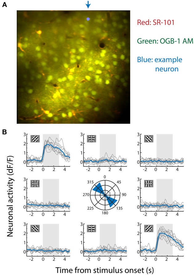
Figure 1
(A) Contrast-enhanced average of all x-y movement-corrected frames recorded from an anesthetized mouse during a two-photon calcium imaging experiment used for decoding. The data were obtained by recor...
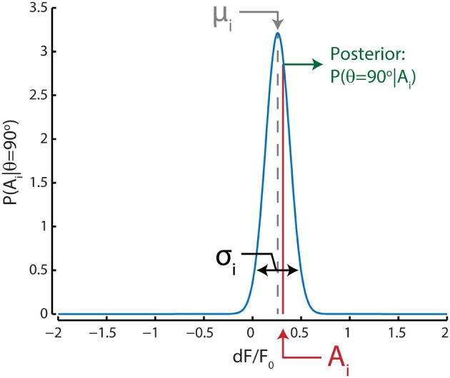
Figure 2
Graphical representation of the Bayesian decoding scheme shows the process for one example neuron i for a single stimulus direction (90u00b0) in one test trial . The probability of responses to a 90u0...
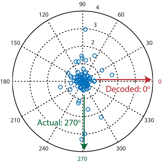
Figure 3
Example decoding trial where the population vector algorithm fails to decode the presented stimulus direction . Each blue circle in the polar plot is a single neuron where its preferred direction is r...
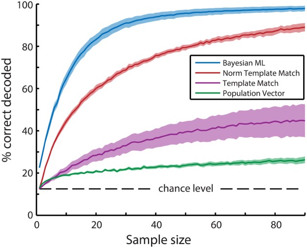
Figure 4
Mean bootstrapped performance over all recordings ( N = 6) reveals superior performance of the Bayesian maximum-likelihood (ML) direction decoding algorithm . Bootstrapping was performed with 100 rand...
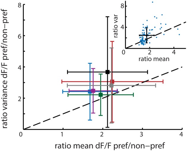
Figure 5
Main figure shows the mean and standard deviation per recording session ( n = 6 animals) in ratio variance (y-axis) and ratio mean (x-axis) activation level differences between time bins corresponding...
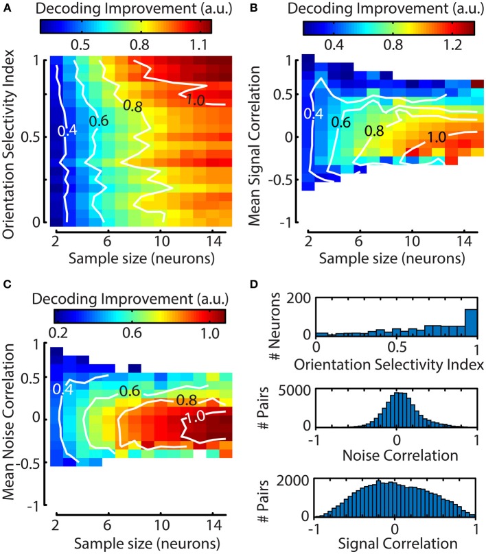
Figure 6
The contribution of a single neuron to the decoding performance of a Bayesian ML algorithm depends on the neuron's orientation selectivity index (OSI) and its mean correlation with other neurons . (Au...
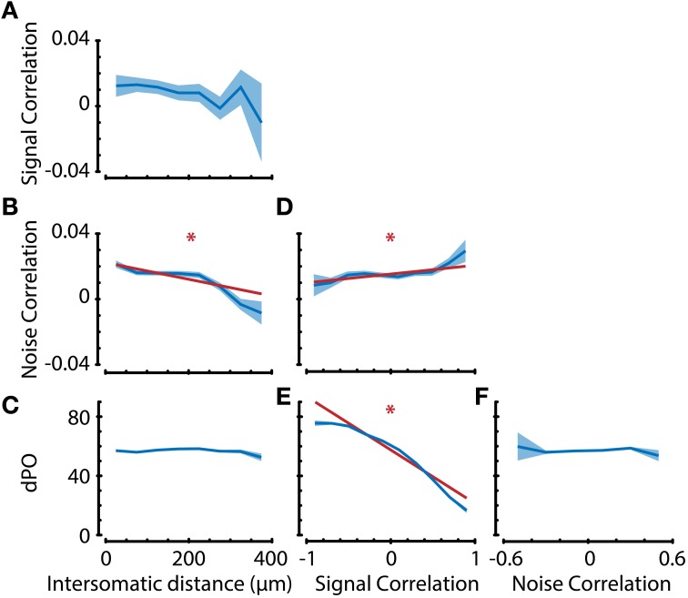
Figure 7
Analysis of interdependence between response properties suggests dissociation in anatomical substrates of noise correlations and preferred orientation . (Au2013F) Neuronal property interdependence ana...
Figure images are served from the NIH/NLM PubMed Central Open Access Subset or Europe PMC; copyright remains with the publishers and authors.
💬 Discussion
0 commentsNo comments yet. Be the first to start a discussion!
Leave a Comment