Abstract
Genetic and chemical perturbations impact diverse cellular phenotypes, including multiple indicators of cell health. These readouts reveal toxicity and antitumorigenic effects relevant to drug discovery and personalized medicine. We developed two customized microscopy assays, one using four targeted reagents and the other three targeted reagents, to collectively measure 70 specific cell health phenotypes including proliferation, apoptosis, reactive oxygen species, DNA damage, and cell cycle stage. We then tested an approach to predict multiple cell health phenotypes using Cell Painting, an inexpensive and scalable image-based morphology assay. In matched CRISPR perturbations of three cancer cell lines, we collected both Cell Painting and cell health data. We found that simple machine learning algorithms can predict many cell health readouts directly from Cell Painting images, at less than half the cost. We hypothesized that these models can be applied to accurately predict cell health assay outcomes for any future or existing Cell Painting dataset. For Cell Painting images from a set of 1500+ compound perturbations across multiple doses, we validated predictions by orthogonal assay readouts. We provide a web app to browse predictions: http://broad.io/cell-health-app. Our approach can be used to add cell health annotations to Cell Painting datasets.
🔬 Techniques
💻 Software
✨ Fluorophores
🧪 Sample Preparation
🔬 Cell Lines
🏭 Microscope Brands
🧪 Reagent Suppliers
💻 Software Details
💻 Code & Software
Python package for image-based profiling
Predicting Cell Health with Morphological Profiles
Processed Cell Painting Data for the LINCS Drug Repurposing Project
💾 Data Repositories
🏛️ Research Organizations (ROR)
Affiliated research institutions:
📋 Methods
CRISPR constructs used for knockout
We performed a CRISPR and CRISPR-associated protein 9 (Cas9) knockout experiment to perturb cells (CRISPR-Cas9). We designed guides to target 59 different genes with an average of two guides per gene (Supplemental Table S1). All sgRNAs were selected from the Avana library ( Doench et al. , 2016 ; Meyers et al. , 2017 ) or by using CRISPick ( https://broad.io/crispick ; Hanna and Doench, 2020 ). Nevertheless, it is important to note that the identity of the CRISPR gene target is not used in training the machine learning models.
Cell lines
We performed CRISPR knockout in three different cell lines (A549, ES2, and HCC44). All cell lines used were stably expressing Cas9 and were part of the Achilles project ( Meyers et al ., 2017 ). Prior to data collection, we confirmed cell line identity using single nucleotide polymorphism (SNP) profiling. We confirmed that all cell lines were mycoplasma negative by using MycoAlert Mycoplasma detection kits (Lonza, Walkersville, MD).
Lentiviral infection and plating
Virus was prepared in 96-well plates according to the published protocol ( https://portals.broadinstitute.org/gpp/public/resources/protocols ). Before initiating the screen, we optimized the number of cells per well and polybrene concentration for each Cas9-expressing cell line. Ultimately, we plated A549, ES2, and HCC44 cells with starting densities of 350, 375, and 150 cells per well, respectively, in 384-well black-wall, clear-bottom plates (Corning Costar). We also optimized sgRNA lentivirus volume to achieve 100% infection while maintaining low toxicity. For the screen, we spin-infected cells with 4 µg/ml polybrene concentration at the optimized density and virus volume ( Aguirre et al. , 2016 ). Three parallel plates were seeded per cell line. On one plate, cells were treated with or without 2 µg/ml puromycin 24 h postinfection, and cell viability was determined using CellTiterGlo (Promega) after 96 h of selection to determine infection efficiency. The second and third plates were used for the Cell Health assays (cell cycle and viability). Cell Painting: cell staining and image acquisition We followed the traditional Cell Painting protocol to acquire the readouts ( Bray et al. , 2016 ). We treated the cells with CRISPR guide perturbations and incubated for 4 d. Following the incubation period, we fixed cells with 10 µl of 16% (wt/vol) methanol-free paraformaldehyde for a final concentration of 3.2% (vol/vol). We imaged cells with a PerkinElmer Opera Phenix confocal HCI microscope at 20× magnification. We applied the standard panel of Cell Painting dyes to mark various cellular compartments: Hoechst 33342 to mark DNA; Concanavalin A/Alexa 488 to mark endoplasmic reticulum (ER); SYTO 14 to mark the nucleoli; cytoplasmic RNA, Phalloidin/Alexa 568, and wheat-germ agglutinin/Alexa 555 to mark actin cytoskeleton, golgi, and plasma membrane (AGP); and MitoTracker Deep Red/Alexa 647 to mark mitochondria ( Bray et al. , 2016 ). We collected nine images per well in five different channels for these different unbiased stains. In total, we collected 138,226 pictures after quality control filtering, which includes five channels per site, nine sites per well, across nine 384-well plates. In total, this represents about 2 TB of images. We deposited raw and illumination-corrected images to the Image Data Resource ( https://idr.openmicroscopy.org ) under accession number idr0080 ( Williams et al. , 2017 ). Cell Painting: image processing The next step in a Cell Painting protocol is to extract morphology features from the images that can be used as an unbiased systems biology measurement to describe how each perturbation impacts various cellular compartments in the assay. We built a CellProfiler image analysis and illumination correction pipeline (version 2.2.0) pipeline to extract these image-based features ( McQuin et al. , 2018 ). We include the CellProfiler pipelines in our github repository. Using the CellProfiler pipeline, we first performed several adjustments to account for potential confounding factors such as background intensity and illumination correction. Next, we used our pipeline to segment cells, distinguish between nuclei and cytoplasm, and then measure specific features related to the various channels captured. We measured the fluorescence intensity, texture, granularity, density, location, and various other measurements for each single cell (see http://cellprofiler-manual.s3.amazonaws.com/CellProfiler-3.0.0/index.html for more details). Following the image analysis pipeline, we obtain 8,964,210 cells and 1785 feature measurements across 9 different plates. We provide the raw output single-cell profiles as extracted from our CellProfiler pipeline on figshare ( Way et al. , 2019 ). Cell Painting: image-based profiling After the image analysis pipeline, the next step is to process the single-cell image-based features that are output of the CellProfiler pipeline. We used a standard approach ( Caicedo et al. , 2017 ) to process the single-cell profiles. First, we aggregated all single cells grouped by perturbation (effectively, by well) by computing the median value per morphology feature. This process takes all single cells and computes a single perturbation profile that is used to compare all perturbations against each other downstream. Next, using the median and median absolute deviation of feature values from empty wells as the center and scale parameters respectively, we normalized all perturbation profiles by subtracting the center and dividing by the scale and did so for each plate independently. This normalization procedure transforms all features to exist on the same scale and enables the perturbation profiles to be compared across plates and batches. We then applied a feature selection procedure to reduce noisy and retain the most informative features. We removed features with missing values in any profile, features with low variance, features with extreme outlier values, and blocklisted features. Extreme outlier features are defined by having measurements greater than 15 SD following normalization. The blocklisted features are generally unreliable features that are known to be noisy and have caused numerical issues in previous experiments ( Way, 2019 ). We used pycytominer ( https://github.com/cytomining/pycytominer ) to perform the profiling pipeline, which can be reproduced at https://github.com/broadinstitute/cell-health . Following these procedures we derived profiles for 357 perturbations representing 119 guides measured across the three different cell lines. We also computed the perturbation consensus signatures of the Cell Painting data (see Materials and Methods : forming consensus signatures ). Our final Cell Painting dataset had 357 consensus profiles measured by 952 morphology features (357 × 952). These data are available on github https://github.com/broadinstitute/cell-health/tree/master/1.generate-profiles/data/profiles . Cell Health assays: cell staining and image acquisition We treated all cells with a panel of specific reagents, each measuring a different aspect of cell health (see Supplemental Table S2). The seven reagents include unbiased dyes, click chemistry, and specific antibody treatments. The reagents measure various aspects of cell health including proliferation, mitosis, DNA damage, reactive oxygen species (ROS), and apoptosis timing. We collected a minimum of four replicates per treatment. Because many reagents fluoresce in different emission spectra, we applied the reagents in parallel. We applied a series of semimanual gating strategies to isolate specific cell health phenotypes in specific cell subsets (Supplemental Table S3). Together, we refer to the collection of measurements as the “Cell Health” assays. More specifically, we collect the Cell Health assay data in a series of two distinct panels: cell cycle and viability. In the first panel we measure Hoechst, EdU, PH3, and gH2AX and use these measurements to quantify cell cycle and DNA damage in specific cell cycle subsets. In the second panel, we measure viability phenotypes using Caspase 3/7, DRAQ7, CellRox, and DPC nucleus morphology measurements. We acquired all cell images using an Opera Phenix HCI Instrument (PerkinElmer) with a 20× water objective (a numerical aperture of 1.0) in confocal mode. We acquired images in four channels using default excitation/emission combinations: for the blue channel (Hoechst) 405/435–480; for the green channel (Alexa 488 and CellEvent), 488/500–550; for the orange channel (Alexa 568 and CellRox Orange), 561/570–630; and for the far red channel (Alexa 647 and DRAQ7), 640/650–760. We applied the Cell Health reagents for cell viability and for cell cycle in two separate plates. The first set of plates ( n = 3 replicate plates) measures cell cycle. We added 5-ethynyl-2′-deoxyuridine (EdU) in live cells for S phase cells to integrate. We then fixed the cells with 4% formaldehyde using standard approaches and detected EdU using Click-iT EdU Alexa Fluor 647 HCS Assay (ThermoFisher C10357 ) according to the vendor protocol. We then performed standard immunofluorescence staining with two antibodies: one targeting phosphohistone H3 (PH3) to measure cells undergoing mitosis and one to identify DNA damage foci in nuclei via γ H2Ax. We followed these PH3 and γ H2Ax antibody treatments by secondary antibodies conjugated with Alexa 488 and Alexa 568, respectively. We added Hoecsht 33342 dye to stain nuclear DNA. For the cell cycle plate, we acquired nine fields of view per well. The second set of plates ( n = 3 replicate plates) measures cell viability. We added CellEvent Caspase-3/7 Green Detection Reagent (ThermoFisher), DRAQ7, and CellROX Orange Reagent (ThermoFisher) dyes to measure apoptotic cells, dead cells, and ROS, respectively. We acquired one field of view per well using green, orange, and far red fluorescence channels as well as brightfield and DPC channels. The cells were incubated at 37°C. Cell Health assays: image analysis We developed and ran two distinct image analysis pipelines in Harmony software (version 4.1; PerkinElmer) for each of the Cell Health plates. Individually for each cell line assayed, and for both cell cycle and cell viability plates, we established a series of manual gating strategies to identify distinct cell line subpopulations (see Figure 1A ). For the cell cycle plate, we performed nucleus segmentation using the Hoechst channel and discarded all nuclei that were at the field border. We identified cells in specific cell cycle stages using Hoechst, Alexa 488 (pH3), and Alexa 647 (EdU) intensities. We identified γ H2AX spots within nuclei based on the Alexa 568 channel. These strategies are standard in the field ( Aguirre et al. , 2016 ). More specifically, we identified subpopulations based on the respective channel intensities and morphological properties for each nucleus as specified: We stratified populations “polyploid,” “polynuclear (large not round nuclei),” and “cells selected for cell cycle” based on total intensity of the Hoechst channel (DNA content) and nucleus “roundness” measurements as output from the PerkinElmer Harmony software. We identified four subpopulations within the “cells selected for cell cycle” population as follows: a) “G1 cells:” selected based on low total Hoechst intensity and low green (pH3) and far red (EdU) channels. We excluded outlier nuclei with unusually high intensity of Hoechst max. b) “G2 cells:” selected based on high total Hoechst intensity and low green (pH3) and far red (EdU) channels. We excluded outlier nuclei with unusually high intensity of Hoechst max. c) “G2/M cells”: selected based on the same criteria as for G2, except we included nuclei with high green (pH3) mean. d) “M cells”: selected based on high green (pH3) mean. e) “S cells”: selected based on high mean far red (EdU) channel intensity. We counted orange spots ( γ H2AX) representing DNA damage loci in each of the cell cycle subpopulations. We determined high γ H2AX activity if there were more than three spots per nucleus. For the cell viability plate, we performed cell segmentation based on the cumulative DPC channels. Again, we identified specific subpopulations based on the following channel intensities: We separated “Dead Cells” and “Live Cells” based on max intensity far red channel (DRAQ7). a) We identified a “Dead Only Cells” subpopulation within the “Dead Cells” population by isolating cells without green (Caspase 3/7) signal. We identified “Caspase Positive Cells” based on green (Caspase 3/7) channel max intensity. a) We distinguished two subpopulations in the “Caspase Positive Cells” named “Early Apoptotic Cells” and “Late Apoptotic Cells” based on low and high far red (DRAQ7) max signal intensity, respectively. We used the mean intensity of the CellROX Orange signal to measure ROS. a) We excluded edge wells in the ROS analysis because of consistent poor signal quality. Additionally, we set these gates for each cell subpopulation using a set of random wells from each cell line and experiment independently. We observed that the intensity measurements used to form the gates were consistent across wells and plates and generally formed distinct cell subpopulation clusters. After using the random wells to set the gates, we used the Harmony microscope software to apply the gates to the remaining wells and plates. We also used CRISPR infection efficiency, which is measured in a separate assay for both cell cycle and viability imaging assays, as negative control features. In total, considering both plates and all cell subpopulations, we measured 70 different variables in the Cell Health Assay. To standardize plate-level differences, we normalized Cell Health readouts per plate by subtracting median values and dividing by the SD. Forming consensus signatures After acquiring the images and processing the data, we prepared the data further before input into our machine learning framework. We generated consensus signatures for each perturbation using a moderated z-score (MODZ) procedure ( Subramanian et al. , 2017 ). Briefly, we calculated pairwise Spearman correlations between all replicates of a single perturbation and then combined profiles by weighting their signature contribution by mean pairwise correlation to all other replicates. We applied this transformation to both Cell Painting profiles and Cell Health assay measurements. We collected more replicates of the Cell Painting data than the Cell Health data. In total, we collected assay readouts from 357 common perturbations (119 CRISPR guides across three cell lines). In the Cell Painting data, we filtered and collapsed 3456 morphology profiles to the common set of 357 consensus profiles. In the Cell Health assays, we filtered and collapsed 2302 well profile readouts to the common set of 357 consensus readouts. We generated consensus signatures because there is no way to match replicate-level information across the assays. We applied UMAP ( McInnes et al. , 2018 ) to the consensus profiles and visualized patterns of ground truth cell health measurements.
Show full methods section
CRISPR constructs used for knockout
We performed a CRISPR and CRISPR-associated protein 9 (Cas9) knockout experiment to perturb cells (CRISPR-Cas9). We designed guides to target 59 different genes with an average of two guides per gene (Supplemental Table S1). All sgRNAs were selected from the Avana library ( Doench et al. , 2016 ; Meyers et al. , 2017 ) or by using CRISPick ( https://broad.io/crispick ; Hanna and Doench, 2020 ). Nevertheless, it is important to note that the identity of the CRISPR gene target is not used in training the machine learning models.
Cell lines
We performed CRISPR knockout in three different cell lines (A549, ES2, and HCC44). All cell lines used were stably expressing Cas9 and were part of the Achilles project ( Meyers et al ., 2017 ). Prior to data collection, we confirmed cell line identity using single nucleotide polymorphism (SNP) profiling. We confirmed that all cell lines were mycoplasma negative by using MycoAlert Mycoplasma detection kits (Lonza, Walkersville, MD).
Lentiviral infection and plating
Virus was prepared in 96-well plates according to the published protocol ( https://portals.broadinstitute.org/gpp/public/resources/protocols ). Before initiating the screen, we optimized the number of cells per well and polybrene concentration for each Cas9-expressing cell line. Ultimately, we plated A549, ES2, and HCC44 cells with starting densities of 350, 375, and 150 cells per well, respectively, in 384-well black-wall, clear-bottom plates (Corning Costar). We also optimized sgRNA lentivirus volume to achieve 100% infection while maintaining low toxicity. For the screen, we spin-infected cells with 4 µg/ml polybrene concentration at the optimized density and virus volume ( Aguirre et al. , 2016 ). Three parallel plates were seeded per cell line. On one plate, cells were treated with or without 2 µg/ml puromycin 24 h postinfection, and cell viability was determined using CellTiterGlo (Promega) after 96 h of selection to determine infection efficiency. The second and third plates were used for the Cell Health assays (cell cycle and viability). Cell Painting: cell staining and image acquisition We followed the traditional Cell Painting protocol to acquire the readouts ( Bray et al. , 2016 ). We treated the cells with CRISPR guide perturbations and incubated for 4 d. Following the incubation period, we fixed cells with 10 µl of 16% (wt/vol) methanol-free paraformaldehyde for a final concentration of 3.2% (vol/vol). We imaged cells with a PerkinElmer Opera Phenix confocal HCI microscope at 20× magnification. We applied the standard panel of Cell Painting dyes to mark various cellular compartments: Hoechst 33342 to mark DNA; Concanavalin A/Alexa 488 to mark endoplasmic reticulum (ER); SYTO 14 to mark the nucleoli; cytoplasmic RNA, Phalloidin/Alexa 568, and wheat-germ agglutinin/Alexa 555 to mark actin cytoskeleton, golgi, and plasma membrane (AGP); and MitoTracker Deep Red/Alexa 647 to mark mitochondria ( Bray et al. , 2016 ). We collected nine images per well in five different channels for these different unbiased stains. In total, we collected 138,226 pictures after quality control filtering, which includes five channels per site, nine sites per well, across nine 384-well plates. In total, this represents about 2 TB of images. We deposited raw and illumination-corrected images to the Image Data Resource ( https://idr.openmicroscopy.org ) under accession number idr0080 ( Williams et al. , 2017 ). Cell Painting: image processing The next step in a Cell Painting protocol is to extract morphology features from the images that can be used as an unbiased systems biology measurement to describe how each perturbation impacts various cellular compartments in the assay. We built a CellProfiler image analysis and illumination correction pipeline (version 2.2.0) pipeline to extract these image-based features ( McQuin et al. , 2018 ). We include the CellProfiler pipelines in our github repository. Using the CellProfiler pipeline, we first performed several adjustments to account for potential confounding factors such as background intensity and illumination correction. Next, we used our pipeline to segment cells, distinguish between nuclei and cytoplasm, and then measure specific features related to the various channels captured. We measured the fluorescence intensity, texture, granularity, density, location, and various other measurements for each single cell (see http://cellprofiler-manual.s3.amazonaws.com/CellProfiler-3.0.0/index.html for more details). Following the image analysis pipeline, we obtain 8,964,210 cells and 1785 feature measurements across 9 different plates. We provide the raw output single-cell profiles as extracted from our CellProfiler pipeline on figshare ( Way et al. , 2019 ). Cell Painting: image-based profiling After the image analysis pipeline, the next step is to process the single-cell image-based features that are output of the CellProfiler pipeline. We used a standard approach ( Caicedo et al. , 2017 ) to process the single-cell profiles. First, we aggregated all single cells grouped by perturbation (effectively, by well) by computing the median value per morphology feature. This process takes all single cells and computes a single perturbation profile that is used to compare all perturbations against each other downstream. Next, using the median and median absolute deviation of feature values from empty wells as the center and scale parameters respectively, we normalized all perturbation profiles by subtracting the center and dividing by the scale and did so for each plate independently. This normalization procedure transforms all features to exist on the same scale and enables the perturbation profiles to be compared across plates and batches. We then applied a feature selection procedure to reduce noisy and retain the most informative features. We removed features with missing values in any profile, features with low variance, features with extreme outlier values, and blocklisted features. Extreme outlier features are defined by having measurements greater than 15 SD following normalization. The blocklisted features are generally unreliable features that are known to be noisy and have caused numerical issues in previous experiments ( Way, 2019 ). We used pycytominer ( https://github.com/cytomining/pycytominer ) to perform the profiling pipeline, which can be reproduced at https://github.com/broadinstitute/cell-health . Following these procedures we derived profiles for 357 perturbations representing 119 guides measured across the three different cell lines. We also computed the perturbation consensus signatures of the Cell Painting data (see Materials and Methods : forming consensus signatures ). Our final Cell Painting dataset had 357 consensus profiles measured by 952 morphology features (357 × 952). These data are available on github https://github.com/broadinstitute/cell-health/tree/master/1.generate-profiles/data/profiles . Cell Health assays: cell staining and image acquisition We treated all cells with a panel of specific reagents, each measuring a different aspect of cell health (see Supplemental Table S2). The seven reagents include unbiased dyes, click chemistry, and specific antibody treatments. The reagents measure various aspects of cell health including proliferation, mitosis, DNA damage, reactive oxygen species (ROS), and apoptosis timing. We collected a minimum of four replicates per treatment. Because many reagents fluoresce in different emission spectra, we applied the reagents in parallel. We applied a series of semimanual gating strategies to isolate specific cell health phenotypes in specific cell subsets (Supplemental Table S3). Together, we refer to the collection of measurements as the “Cell Health” assays. More specifically, we collect the Cell Health assay data in a series of two distinct panels: cell cycle and viability. In the first panel we measure Hoechst, EdU, PH3, and gH2AX and use these measurements to quantify cell cycle and DNA damage in specific cell cycle subsets. In the second panel, we measure viability phenotypes using Caspase 3/7, DRAQ7, CellRox, and DPC nucleus morphology measurements. We acquired all cell images using an Opera Phenix HCI Instrument (PerkinElmer) with a 20× water objective (a numerical aperture of 1.0) in confocal mode. We acquired images in four channels using default excitation/emission combinations: for the blue channel (Hoechst) 405/435–480; for the green channel (Alexa 488 and CellEvent), 488/500–550; for the orange channel (Alexa 568 and CellRox Orange), 561/570–630; and for the far red channel (Alexa 647 and DRAQ7), 640/650–760. We applied the Cell Health reagents for cell viability and for cell cycle in two separate plates. The first set of plates ( n = 3 replicate plates) measures cell cycle. We added 5-ethynyl-2′-deoxyuridine (EdU) in live cells for S phase cells to integrate. We then fixed the cells with 4% formaldehyde using standard approaches and detected EdU using Click-iT EdU Alexa Fluor 647 HCS Assay (ThermoFisher C10357 ) according to the vendor protocol. We then performed standard immunofluorescence staining with two antibodies: one targeting phosphohistone H3 (PH3) to measure cells undergoing mitosis and one to identify DNA damage foci in nuclei via γ H2Ax. We followed these PH3 and γ H2Ax antibody treatments by secondary antibodies conjugated with Alexa 488 and Alexa 568, respectively. We added Hoecsht 33342 dye to stain nuclear DNA. For the cell cycle plate, we acquired nine fields of view per well. The second set of plates ( n = 3 replicate plates) measures cell viability. We added CellEvent Caspase-3/7 Green Detection Reagent (ThermoFisher), DRAQ7, and CellROX Orange Reagent (ThermoFisher) dyes to measure apoptotic cells, dead cells, and ROS, respectively. We acquired one field of view per well using green, orange, and far red fluorescence channels as well as brightfield and DPC channels. The cells were incubated at 37°C. Cell Health assays: image analysis We developed and ran two distinct image analysis pipelines in Harmony software (version 4.1; PerkinElmer) for each of the Cell Health plates. Individually for each cell line assayed, and for both cell cycle and cell viability plates, we established a series of manual gating strategies to identify distinct cell line subpopulations (see Figure 1A ). For the cell cycle plate, we performed nucleus segmentation using the Hoechst channel and discarded all nuclei that were at the field border. We identified cells in specific cell cycle stages using Hoechst, Alexa 488 (pH3), and Alexa 647 (EdU) intensities. We identified γ H2AX spots within nuclei based on the Alexa 568 channel. These strategies are standard in the field ( Aguirre et al. , 2016 ). More specifically, we identified subpopulations based on the respective channel intensities and morphological properties for each nucleus as specified: We stratified populations “polyploid,” “polynuclear (large not round nuclei),” and “cells selected for cell cycle” based on total intensity of the Hoechst channel (DNA content) and nucleus “roundness” measurements as output from the PerkinElmer Harmony software. We identified four subpopulations within the “cells selected for cell cycle” population as follows: a) “G1 cells:” selected based on low total Hoechst intensity and low green (pH3) and far red (EdU) channels. We excluded outlier nuclei with unusually high intensity of Hoechst max. b) “G2 cells:” selected based on high total Hoechst intensity and low green (pH3) and far red (EdU) channels. We excluded outlier nuclei with unusually high intensity of Hoechst max. c) “G2/M cells”: selected based on the same criteria as for G2, except we included nuclei with high green (pH3) mean. d) “M cells”: selected based on high green (pH3) mean. e) “S cells”: selected based on high mean far red (EdU) channel intensity. We counted orange spots ( γ H2AX) representing DNA damage loci in each of the cell cycle subpopulations. We determined high γ H2AX activity if there were more than three spots per nucleus. For the cell viability plate, we performed cell segmentation based on the cumulative DPC channels. Again, we identified specific subpopulations based on the following channel intensities: We separated “Dead Cells” and “Live Cells” based on max intensity far red channel (DRAQ7). a) We identified a “Dead Only Cells” subpopulation within the “Dead Cells” population by isolating cells without green (Caspase 3/7) signal. We identified “Caspase Positive Cells” based on green (Caspase 3/7) channel max intensity. a) We distinguished two subpopulations in the “Caspase Positive Cells” named “Early Apoptotic Cells” and “Late Apoptotic Cells” based on low and high far red (DRAQ7) max signal intensity, respectively. We used the mean intensity of the CellROX Orange signal to measure ROS. a) We excluded edge wells in the ROS analysis because of consistent poor signal quality. Additionally, we set these gates for each cell subpopulation using a set of random wells from each cell line and experiment independently. We observed that the intensity measurements used to form the gates were consistent across wells and plates and generally formed distinct cell subpopulation clusters. After using the random wells to set the gates, we used the Harmony microscope software to apply the gates to the remaining wells and plates. We also used CRISPR infection efficiency, which is measured in a separate assay for both cell cycle and viability imaging assays, as negative control features. In total, considering both plates and all cell subpopulations, we measured 70 different variables in the Cell Health Assay. To standardize plate-level differences, we normalized Cell Health readouts per plate by subtracting median values and dividing by the SD. Forming consensus signatures After acquiring the images and processing the data, we prepared the data further before input into our machine learning framework. We generated consensus signatures for each perturbation using a moderated z-score (MODZ) procedure ( Subramanian et al. , 2017 ). Briefly, we calculated pairwise Spearman correlations between all replicates of a single perturbation and then combined profiles by weighting their signature contribution by mean pairwise correlation to all other replicates. We applied this transformation to both Cell Painting profiles and Cell Health assay measurements. We collected more replicates of the Cell Painting data than the Cell Health data. In total, we collected assay readouts from 357 common perturbations (119 CRISPR guides across three cell lines). In the Cell Painting data, we filtered and collapsed 3456 morphology profiles to the common set of 357 consensus profiles. In the Cell Health assays, we filtered and collapsed 2302 well profile readouts to the common set of 357 consensus readouts. We generated consensus signatures because there is no way to match replicate-level information across the assays. We applied UMAP ( McInnes et al. , 2018 ) to the consensus profiles and visualized patterns of ground truth cell health measurements.
Machine learning framework
We randomly split 15% of the consensus signatures into a separate test set. We balanced this stratification by cell line. We then used the remaining 85% to train all 70 cell health models. In total, we used 303 samples as the training set and 54 as the test set. We elected to train elastic net regression models using sklearn (version 0.20.3) ( Pedregosa et al. , 2011 ; Zou and Hastie, 2005 ). We chose this model because it is quick to train, is easily interpretable, and will induce sparsity in selecting model features. We also trained classification models and binarized training and testing data by using > 1.5 SD away from the mean as positive examples. However, because the classification approach was unstable and sensitive to low sample sizes, we elected to move forward using only the regression models (see https://github.com/broadinstitute/cell-health/issues/78 ). To identify optimal alpha and elastic net mixing parameters, we performed a grid search and fivefold cross-validation using the training set only. For each model independently, we observed cross-validation performance across 9 different alpha parameters ([0.01, 0.1, 0.2, 0.3, 0.4, 0.5, 0.6, 0.7, 0.8]) and 11 different elastic net mixing parameters ([0.1, 0.12, 0.14, 0.16, 0.2, 0.3, 0.4, 0.5, 0.7, 0.8, 0.9]). Alpha controls the regularization penalty term for all features, and the elastic net mixing parameter controls the trade-off between L1 and L2 regression where 0 = L1 and 1 = L2. Therefore, the closer the elastic net mixing parameter is to 0, the sparser the model. We optimized and trained 70 different elastic net regression models for each of the 70 Cell Health assay readouts independently. We repeated this procedure and independently optimized 70 additional models using randomly shuffled data. For the shuffling procedure, we randomly shuffled the Cell Painting features independently per column before training. We use the shuffled model performance as a suitable baseline to compare real model performance.
Machine learning evaluation
We evaluated each of the 70 Cell Health regression models independently using R-squared statistics from sklearn version 0.20.3 ( Pedregosa et al. , 2011 ). We calculated R-squared for the full training and testing partitions, in shuffled training and testing partitions, and for each cell line independently for all 70 models. The measurement can be interpreted as how well the models could predict the real Cell Health readout with values approaching one as perfect fits. It is best to compare test set performance in real versus shuffled data. The test set performance in real data simulates how models are expected to perform in data not used for model training. The shuffled performance indicates if there is any expected performance inflation. Machine learning robustness: investigating the impact of sample size We performed an analysis in which we randomly dropped an increasing amount of samples from the training set before model training. After dropping the predefined number of samples, we retrained all 70 cell health models and assessed performance on the original holdout test set. We performed this procedure 10 times with 10 unique random seeds to mirror a more realistic scenario of new data collection and to reduce the impact of outlier samples on model training. Machine learning robustness: systematically removing feature classes We performed an analysis in which we systematically dropped features measured in specific compartments (Nuclei, Cells, and Cytoplasm), specific channels (RNA, Mito, ER, DNA, and AGP), and specific feature groups (Texture, Radial Distribution, Neighbors, Intensity, Granularity, Correlation, and Area Shape) and retrained all models. We omitted one feature class and then independently optimized all 70 cell health models as described in the Machine learning framework results section above. We repeated this procedure once per feature class. Drug Repurposing Hub Cell Painting data: image-based profiling A subset of the Drug Repurposing Hub compounds ( n = 1571) ( Corsello et al. , 2017 ) were profiled using the Cell Painting assay across about six doses per compound. We processed this dataset using a standard image-based profiling pipeline to extract consensus profiles per treatment. See https://github.com/broadinstitute/lincs-cell-painting for complete details and instructions on how to reproduce. Briefly, we applied a CellProfiler image analysis pipeline to segment cells, adjusted for background intensity, and measured morphology features for three compartments: cells, cytoplasm, and nuclei. The output of this procedure was 136 SQLite files (one for each plate) representing unnormalized single-cell profiles. Next, we developed and applied an image-based profiling bioinformatics pipeline to generate treatment consensus profiles from the single-cell measurements ( Caicedo et al. , 2017 ). The same image analysis pipeline and bioinformatics pipeline were used to process all the plates in the experiment. In the pipeline, we first median-aggregated the single cells by feature to form well profiles and then, using the median and median absolute deviation of feature values from DMSO as the center and scale parameters, respectively, we normalized all perturbation profiles by subtracting the center and dividing by the scale and did so for each plate independently. The plates in this dataset have 24 DMSO-treated wells and therefore represented a good alignment control to adjust for plate level differences. Each plate also has two positive controls (BRD-K50691590 [Bortezomib] and BRD-K60230970 [MG-132]) at 20 mmol/l with 12 replicates each for all plates. We visualized positive and negative control profiles in our UMAP space to determine the extent of technical artifacts present in our data. Following the z-score normalization, we combined all treatment replicates (∼6 per compound and dose pair) using MODZ consensus signatures. We generated consensus profiles for control replicates by well across plate maps. In total, this procedure resulted in 10,752 different treatment profiles and 1788 normalized CellProfiler morphology features. Drug Repurposing Hub Cell Painting data: predicting cell health readouts We applied all Cell Health models to the 10,752 Drug Repurposing Hub consensus Cell Painting profiles. We simply applied the Cell Health trained models using the sklearn model.predict() method. Every feature measured in the CRISPR perturbation Cell Painting profiles were also measured in the Drug Repurposing Hub output. The result of the model application was 70 Cell Health readouts for all 10,752 treatments. We used these predictions for model validation with external data and for visualization in the web app scatter plots. Assessing generalizability of cell health models applied to Drug Repurposing Hub data We used our cell health webapp ( https://broad.io/cell-health-app ) to identify compounds with high predictions for three models with high or intermediate performance: ROS, Number of G1 cells , and Number of gH2AX spots in G1 cells . For each model, we identified classes of compounds with consistently high scores, then tested for statistical enrichment: for proteasome inhibitors in the ROS model, PLK inhibitors in the Number of G1 cells model, and aurora kinase and tubulin inhibitors in the Number of gH2AX spots in G1 cells model. We used one-sided Fisher’s exact tests to quantify differences in expected proportions between high and low model predictions. For each case, we determined high and low predictions based on the 50% quantile threshold for each model independently. Drug Repurposing Hub Cell Painting data: visualization We also applied UMAP to the 10,752 Drug Repurposing Hub Cell Painting profiles and extracted two lower dimensional representations. UMAP reduces the Cell Painting profiles to two features that capture the global structure of the input data. Prior to UMAP transformation, we applied a feature selection procedure to the Drug Repurposing Hub profiles. We removed features with low variance, features with missing values in any consensus profile, blocklisted features ( Way, 2019 ), and features with extreme outlier values defined by greater than 15 SD following normalization. This procedure reduced the feature dimension from 1788 to 572. By reducing the number of features, we can be more confident that the major sources of variation are not biased by CellProfiler feature redundancies or by technical artifacts of sample processing. Drug Repurposing Hub Cell Painting data: dose-response analysis To model dose, we fit Hill equations (4 parameter log-logistic model) to all 1571 Drug Repurposing compounds consensus signatures transformed into each of the 70 different Cell Health model predictions. Before input into the model, we zero-one transformed Cell Health predictions across doses for each compound independently. For most compounds, this normalization procedure happens for six data points (representing six doses per compound consensus signature) at a time. The zero-one procedure assigns a value of zero to the lowest value, one to the highest value, and scales each intermediate value accordingly. This procedure results in 109,970 different model fits. We used the drc R package (version 3.0-1) to fit all models ( Ritz et al. , 2015 ). We present all precomputed dose fit models to be explored at https://broad.io/cell-health-app . Comparing viability predictions to an orthogonal readout We downloaded the PRISM assay results (version 19Q4) from the Cancer Dependency Map website at https://depmap.org/portal/download/ ( Corsello et al. , 2017 ). The PRISM assay measures viability of multiple cell lines in a pooled format and deconvolutes results based on barcoded readouts ( Yu et al. , 2016 ). We focused on the A549 cell line and compounds that were measured in both the PRISM assay and the Drug Repurposing collection. The PRISM assay profiled 1382 of the 1571 Drug Repurposing Compounds. The PRISM assay also used slightly different doses than the Drug Repurposing Hub collection procedure. Therefore, to align doses, we converted doses into dose ranks and report Spearman correlations between the two datasets (see Figure 4A ).
Code and data availability
All data and code are publicly available. Analysis software to reproduce the full paper is available at https://github.com/broadinstitute/cell-health/tree/v2.0 ( Way et al. , 2020 ). Raw and illumination-corrected Cell Painting images are available in the Image Data Resource (accession number idr0080). Single cell morphology profiles derived from these images are available at the National Institutes of Health (NIH) Figshare at https://doi.org/10.35092/yhjc.9995672.v5 . Processed Cell Painting profiles and raw and processed Cell Health readouts are also available at https://github.com/broadinstitute/cell-health/tree/v2.0 . Processing code and data for the Cell Painting Drug Repurposing Hub data is available at https://github.com/broadinstitute/lincs-cell-painting/tree/v0.1 .
Cell Health predictions for the Drug Repurposing
Hub compounds are available to explore at https://broad.io/cell-health-app .
Supplementary Material Click here for additional data file. Click here for additional data file. Click here for additional data file. Click here for additional data file. Click here for additional data file.
📊 Figures
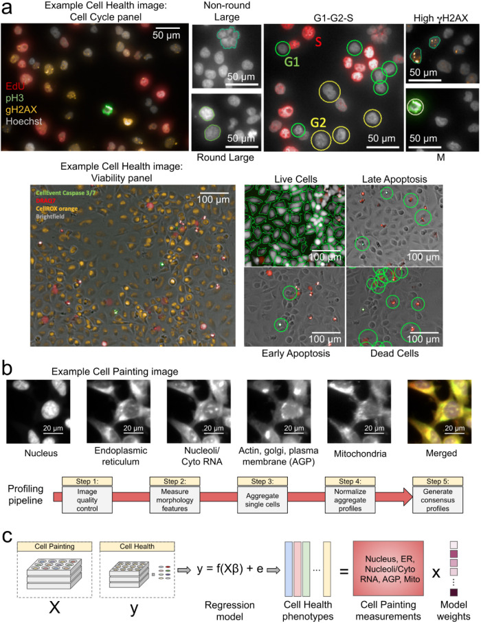
FIGURE 1:
Data processing and modeling approach. (a) Example images and workflow from the Cell Health assays. We apply a series of manual gating strategies (see Materials and Methods ) to isolate cell subpopula...
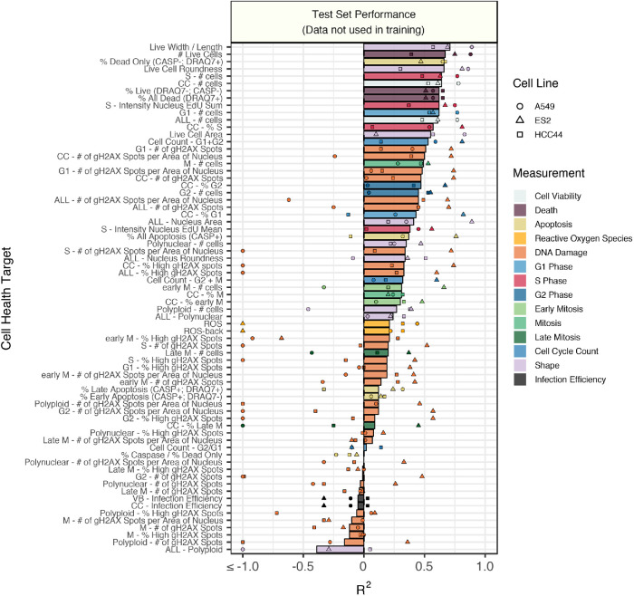
FIGURE 2:
Test set model performance of predicting 70 Cell Health readouts with independent regression models. Performance for each phenotype is shown, sorted by decreasing R 2 performance. The bars are colored...
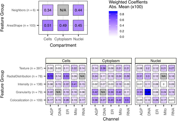
FIGURE 3:
The importance of each class of Cell Painting features in predicting 70 Cell Health readouts. Each square represents the mean absolute value of model coefficients weighted by test set R 2 across every...
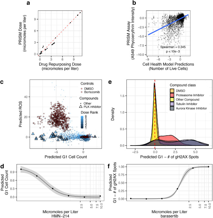
FIGURE 4:
Validating Cell Health models to Cell Painting data from The Drug Repurposing Hub. The models were not trained using the Drug Repurposing Hub data. (a) The results of the dose alignment between the PR...
Figure images are served from the NIH/NLM PubMed Central Open Access Subset or Europe PMC; copyright remains with the publishers and authors.
💬 Discussion
0 commentsNo comments yet. Be the first to start a discussion!
Leave a Comment