Abstract
The microenvironment determines cell behavior, but the underlying molecular mechanisms are poorly understood because quantitative studies of cell signaling and behavior have been challenging due to insufficient spatial and/or temporal resolution and limitations on microenvironmental control. Here we introduce microenvironmental selective plane illumination microscopy (meSPIM) for imaging and quantification of intracellular signaling and submicrometer cellular structures as well as large-scale cell morphological and environmental features. We demonstrate the utility of this approach by showing that the mechanical properties of the microenvironment regulate the transition of melanoma cells from actin-driven protrusion to blebbing, and we present tools to quantify how cells manipulate individual collagen fibers. We leverage the nearly isotropic resolution of meSPIM to quantify the local concentration of actin and phosphatidylinositol 3-kinase signaling on the surfaces of cells deep within 3D collagen matrices and track the many small membrane protrusions that appear in these more physiologically relevant environments.
🔬 Techniques
🧬 Organisms
✨ Fluorophores
🧪 Sample Preparation
🔬 Cell Lines
🏭 Microscope Brands
🧪 Reagent Suppliers
🔴 Lasers
📷 Detectors
💻 Software Details
🏛️ Research Organizations (ROR)
Affiliated research institutions:
📋 Methods
Microscope Design
A detailed illustration of the optical setup can be found in Figures 7A–7C and a detailed parts list and drawings of custom components as well as an instruction on the microscope alignment is located in the in the meSPim Supplemental Information zip file . Near infrared laser pulses (150 fs pulse length, 80 MHz repetition rate, wavelength 900 nm) from a Ti:Sapph oscillator (Chameleon Ultra II, Coherent) were expanded five times by a Galilean telescope and shaped to a Bessel beam by an Axicon (Thorlabs). Following an achromatic lens, the resulting ring-shaped intensity distribution in a Fourier plane was cleaned up with a custom-made photomask (Photosciences). The mask contained a series of thin annuli that varied slightly in inner and outer diameter to adjust the desired propagation length and optimize light transmission (around 70% for the design wavelength of 900 nm). The mask is necessary to clean up optical imperfections of the Axicon. The ring was imaged onto a first galvanometric mirror (Cambridge Technology), which scans the Bessel beam in the lateral plane. The ring image was further relayed with two telecentric scan lenses (Sill Optics) to a second galvanometric mirror (Cambridge Technology), which performed the axial scan, and was subsequently imaged into the backfocal plane of the illumination objective with a scan lens (Sill Optics) and a tube lens (ITL200, Thorlabs). Folding mirrors were used to very slightly adjust the rotation of the scan axes relative to the Cartesian axes that span the imaging volume. Nikon NA 0.8/40X water dipping objectives were used for illumination and fluorescence detection, arranged orthogonally to each other. The detection objective was actuated by a piezo actuator (PiFOC, Physik Instrumente) to perform z-stepping for 3D image acquisition. Fluorescence light collected by the detection objective was split into a green and red channel by a dichroic mirror (Chroma) and imaged with tube lenses (ITL 200, Thorlabs) on two sCMOS cameras (Orca Flash II, Hamamatsu). Excitation light was blocked by two short-pass filters (Semrock). Instrument control was performed by a custom written LabView code developed by Coleman Technologies. The initial software kernel was licensed from Howard Hughes Medical Institute’s Janelia Farm (HHMI). The kernel was then substantially expanded by Coleman Technologies to suit our microscope and add additional functionalities such as the descanned mode. The entire code package can be requested for academic use from the corresponding authors and will be delivered under material transfer agreements with HHMI and UT Southwestern Medical Center. In the normal mode, the Bessel beam was laterally scanned five times using a triangular waveform during the acquisition of one image frame. In the descanned mode, the cameras were operated in the light sheet mode and a single scan of the Bessel beam, tightly synchronized to the camera readout, was performed during the acquisition of one image frame.
Show full methods section
Microscope Design
A detailed illustration of the optical setup can be found in Figures 7A–7C and a detailed parts list and drawings of custom components as well as an instruction on the microscope alignment is located in the in the meSPim Supplemental Information zip file . Near infrared laser pulses (150 fs pulse length, 80 MHz repetition rate, wavelength 900 nm) from a Ti:Sapph oscillator (Chameleon Ultra II, Coherent) were expanded five times by a Galilean telescope and shaped to a Bessel beam by an Axicon (Thorlabs). Following an achromatic lens, the resulting ring-shaped intensity distribution in a Fourier plane was cleaned up with a custom-made photomask (Photosciences). The mask contained a series of thin annuli that varied slightly in inner and outer diameter to adjust the desired propagation length and optimize light transmission (around 70% for the design wavelength of 900 nm). The mask is necessary to clean up optical imperfections of the Axicon. The ring was imaged onto a first galvanometric mirror (Cambridge Technology), which scans the Bessel beam in the lateral plane. The ring image was further relayed with two telecentric scan lenses (Sill Optics) to a second galvanometric mirror (Cambridge Technology), which performed the axial scan, and was subsequently imaged into the backfocal plane of the illumination objective with a scan lens (Sill Optics) and a tube lens (ITL200, Thorlabs). Folding mirrors were used to very slightly adjust the rotation of the scan axes relative to the Cartesian axes that span the imaging volume. Nikon NA 0.8/40X water dipping objectives were used for illumination and fluorescence detection, arranged orthogonally to each other. The detection objective was actuated by a piezo actuator (PiFOC, Physik Instrumente) to perform z-stepping for 3D image acquisition. Fluorescence light collected by the detection objective was split into a green and red channel by a dichroic mirror (Chroma) and imaged with tube lenses (ITL 200, Thorlabs) on two sCMOS cameras (Orca Flash II, Hamamatsu). Excitation light was blocked by two short-pass filters (Semrock). Instrument control was performed by a custom written LabView code developed by Coleman Technologies. The initial software kernel was licensed from Howard Hughes Medical Institute’s Janelia Farm (HHMI). The kernel was then substantially expanded by Coleman Technologies to suit our microscope and add additional functionalities such as the descanned mode. The entire code package can be requested for academic use from the corresponding authors and will be delivered under material transfer agreements with HHMI and UT Southwestern Medical Center. In the normal mode, the Bessel beam was laterally scanned five times using a triangular waveform during the acquisition of one image frame. In the descanned mode, the cameras were operated in the light sheet mode and a single scan of the Bessel beam, tightly synchronized to the camera readout, was performed during the acquisition of one image frame.
Cell Culture and Reagents
MV3 and A375 melanoma cells were cultured using DMEM (Gibco) supplemented with 10% fetal bovine serum (FBS) at 5% CO 2 and 21% O 2 . Primary melanoma cells were cultured using the Primary Melanocyte Growth Kit (ATCC) at 5% CO 2 . HBECs immortalized with Cdk4 and hTERT expression and transformed with p53 knockdown, Kras V12 , and cMyc expression ( Sato et al., 2013 ) were cultured in keratinocyte serum-free medium (Gibco) supplemented with 50 mg/ml of bovine pituitary extract (Gibco), 5 ng/ml of EGF (Gibco), and 1% Anti-Anti (Gibco) in a humidified incubator at 5% CO 2 , 2% O 2 , and 37° C. To induce formation of tumor spheres, cells were seeded into ultra-low attachment round-bottom 96-well plates (Corning) at a density of 10,000–30,000 cells per well for 2–4 days before imaging. The GFP-tractin construct contains residues 9–52 of the enzyme IPTKA ( Johnson and Schell, 2009 ) fused to GFP ( Yi et al., 2012 ). The CyOFP-tractin peptide contains the tractin peptide fused to the novel CyOFP protein. CyOFP is a cyan-excitable orange fluorescent protein with peak excitation at 505 nm and peak emission at 588 nm, details of which will be described in a separate article currently in preparation. The td-Tomato membrane marker contains td-Tomato fused to the first 60 base pairs of GAP43 (neuromodulin). The GFP membrane marker contains GFP fused to the 20-amino acid farnesylation signal from c-Ha-Ras ( Kanchanawong et al., 2010 ). The GFP-Kras V12 plasmid was constructed by cloning a Kras V12 fragment from the pLenti-Kras V12 construct ( Sato et al., 2013 ) into the pLVX-GFP vector (Clontech). Fluorescent protein constructs were expressed in cells using the pLVX lentiviral system (Clontech) according to the manufacturer’s instructions, except for the GFP membrane marker, which was expressed using Lipofectamine (Invitrogen). The collagen matrix was labeled with the collagen-binding peptide, CNA35 ( Xu et al., 2004 ), that had been expressed in Escherichia coli , purified, and fluorescently tagged using N-hydroxysuccinimide-ester chemistry (Cy5, Amersham). Collagen gels were created by mixing either rat tail collagen I (Corning) or bovine collagen I (Advanced Biomatrix) with concentrated PBS and water to create gels of either 2.4 mg/ml or 2.0 mg/ml, respectively. This collagen solution was then neutralized with 1 N NaOH and mixed with cells just prior to incubation at 37° C to induce collagen polymerization. For the indicated experiments, blebbistatin (Sigma) was added to the collagen/cell mixture at a final concentration of 20 μM prior to collagen polymerization. Melanoma cells imaged near glass were embedded in an identical mixture of cells and collagen matrix polymerized in glass-bottom 96-well dishes (PerkinElmer). Confocal image stacks were acquired using a 60× (CFI Apo TIRF) objective on a Nikon Eclipse Ti microscope fitted with a Yokagawa spinning disk scan unit and Andor iXon emCCD camera.
Microscope Sample Preparation
The sample holder was prepared by heating 2% agarose with water, then solidifying this mixture in a custom mold ( Figures 7B and 7C ) to attach the agar sample holder to a stage-mounted dovetail. Once solidified, the sample holder was submerged in imaging medium before addition of the cell/collagen mixture. The imaging medium was either phenol red-free DMEM supplemented with 10% FBS or Leibovitz’s L15 medium supplemented with 10% FBS for the melanoma or HBEC cells, respectively. 3D Image Rendering All 3D volume renderings were performed using ImageJ (NIH), and all 3D surface renderings were performed using MATLAB (Mathworks). Image brightness and contrast were linearly adjusted prior to volume rendering. Since noise can obscure other features in 3D renderings, we median filtered the spheroid in Figure 2D , with a kernel radius of 1 pixel, and the cell in Figure 4B , with a kernel radius of 4 pixels. Segments of Movie S3 , frames from which appear in Figures 4B and 4E , were also corrected for photobleaching by fitting the intensity of each cell over time to a decaying double exponential ( Hodgson et al., 2006 ) and then normalizing the image intensity by the fit.
Optical Sectioning Characterization and Image Deconvolution
Optical sectioning in the axial direction for descanned and normal imaging modes was measured as described previously ( Dean et al., 2015 ). Images were deconvolved as follows unless otherwise noted ( Figure S6 ). The PSF was measured by ensemble averaging the 3D images of five individual 100 nm fluorescent nanospheres. We rotationally averaged the PSF about the axial direction to reduce noise. Using the averaged PSF we performed Wiener deconvolution ( Sibarita, 2005 ). For cytoplasmically labeled cells, the Wiener parameter was estimated from each 3D frame following a rough segmentation of the cell. The signal was then measured as the average fluorescence intensity located within the cell and more than 5 pixels away from the cell boundary, and the noise was measured as the SD of the intensity located outside the cell and more than 20 pixels away from the cell boundary. Following the deconvolution, the images were apodized with an apodization filter that was defined by smoothing and then thresholding the optical transfer function (OTF) in the spatial frequency domain. The filter had a value of 1 at the origin and 0 at the boundary of the filter support volume determined by the OTF voxels above threshold. In between, the filter decayed linearly. The threshold value, which we term apodization height, was set by the user as a percentage (see below) of the maximum value of the OTF.
Characterization of Collagen Fibers
Collagen fibers were detected with 3D steerable curve filters ( Aguet et al., 2005 ; González et al., 2009 ; Jacob and Unser, 2004 ). We performed multiscale detection by combining curve filters of widths 2–5 pixels. After filtering, the fiber skeletons were obtained by non-maximum suppression of the filter response. In Figure 3C the local fiber density was measured at every pixel as the percentage of fiber pixels retained after non-maximum suppression and thresholding that fell within a spherical volume of radius ~2 μm. This measure is readily interpretable as the local pixel occupancy of the thresholded non-maximum suppression image. The volume within the cell was excluded from the occupancy analysis and all pixels with local occupancies above 0.015 appear white. In Figure 3F , we measured the mean fiber density as a function of distance from the cell edge without locally smoothing the fiber density. Fiber alignment toward the cell center was characterized by the nematic order parameter ( Chaikin and Lubensky, 2000 ), which in three dimensions is (Equation 1) S = 〈 P 2 ( cos θ ) 〉 = 〈 3 cos 2 θ − 1 2 〉 , where P 2 is the second order Legendre polynomial, and θ is the angle between the fiber alignment and the director, which we define here as the direction toward the cell center. Fibers aligned toward the cell center will have a nematic order parameter of 1, randomly aligned fibers will have an order parameter of 0, and those aligned in the plane perpendicular to the direction toward the cell center will have an order parameter of −1/2. Figure 3F shows the nematic order parameter as a function of distance from the cell edge, whereas for simplicity Figure 3E shows only cos θ , i.e., the dot product of the fiber alignment with the director. In Figure 3E , a value of 1 then indicates that the fiber is aligned toward the cell center and a value of 0 indicates that the fiber is perpendicular to the direction toward the cell center.
Cell Segmentation
Fluorescence movies of cytoplasmically labeled cells were deconvolved as described above. An apodization height of 0.05 was used for movies from which we measured bleb areas, whereas an apodization height of 0.07 was used for movies from which we tracked blebs since those movies were taken with a shorter exposure time. To preserve surface features, lower apodization heights were used for movies for which we calculated surface intensities. For each 3D image, we segmented cells by calculating first an Otsu threshold level, followed by a grayscale flood-fill operation, removal of small objects disconnected from the cell, and creation of an isosurface at the intensity level specified by the threshold ( Figures 7D–7G ) ( Otsu, 1979 ). Mathematically, the isosurface is a triangulated mesh with each triangular face adjacent to one other face at each of its sides. We used MATLAB’s isosurface function to generate the mesh from the processed image. Then we slightly smoothed the mesh geometry using curvature flow ( Desbrun et al., 1999 ). For images with multiple cells, we separately calculated an Otsu threshold level for each cell. The intensity histogram of an image with multiple cells tends to be composed of multiple signal peaks (the cells) and multiple background peaks, since the background intensity induced by the beam changes upon interacting with a cell. To threshold the foreground, we therefore calculated the corner intensity of the cumulative distribution function (CDF) of the pixel intensities. We defined the corner intensity as the intensity at which the CDF is closest to the coordinate corresponding to a pixel intensity of 0 and a cumulative probability of 1. This approach assumes that the large number of pixels in background intensity distributions are more narrowly banded in their intensity values than the more heterogeneous foreground intensity distributions. Using this corner value for a coarse foreground thresholding, we morphologically dilated each foreground connected component separately, and then calculated an Otsu threshold for each dilated region.
Bleb Detection and Tracking
Blebs are characterized by uniform or regular curvature. We measured the mean curvature at each triangular face as described in previous work ( Figure S7G ) ( Elliott et al., 2015 ). Since curvature can be noisy, we median filtered surface curvature in 3D with a kernel radius of 1 pixel. We then further smoothed curvature by creating a graph of adjacent faces and smoothing curvature over the graph for 12 iterations, (Equation 2) S = ( A 3 ) k C , where S is the smoothed curvature, A is the adjacency matrix of the faces graph, k is the number of smoothing iterations, and C is the curvature. To detect blebs, we performed a watershed segmentation of curvature over the graph of triangular faces ( Figure 7H ) ( Mangan and Whitaker, 1999 ). The watershed algorithm oversegments blebs. We merged adjacent watershed regions in two different ways. First, in each frame we calculated the Otsu threshold level of smoothed mean curvature defined over the faces and labeled any watershed region that did not include a face with a curvature above the threshold as a flat region. For each non-flat region, we then calculated the spill depth ( Mangan and Whitaker, 1999 ), defined as the largest curvature within the region minus the largest curvature at its boundary. The boundary of a region is composed of both the faces in the region that are adjacent to a non-flat region and the immediately adjacent faces in neighboring non-flat regions. We also defined the spill neighbor as the adjacent region with the largest curvature on the boundary. Starting with the greatest spill depth, we iteratively merged regions with their spill neighbors until no spill depth was greater than 0.6 times the Otsu curvature threshold. We next merged adjacent regions by analyzing their configuration in 3D. For each region, including those labeled flat, we measured the closure surface area, σ , defined as the additional surface area needed to close the portion of the mesh occupied by the region. First we found the vertices at the edge of the region and calculated the mean position, v m , of those vertices. Next, we closed the mesh by connecting the faces at the edge of the region to the vertex v m . We next iteratively merged pairs of adjacent regions if the following condition was met, (Equation 3) σ A + σ B − σ A B σ A σ B > ρ , where σ A and σ B are the closure surface areas of the two considered regions, σ AB is the closure surface area of the two merged regions, and ρ is a parameter specified by the user. Here we used a r of 0.3. This condition is analogous to the law of cosines, and can be understood intuitively as merging pairs of regions that form a large angle relative to one another. A non-flat region was allowed to merge with either a non-flat or flat region, but two flat regions were not allowed to merge. To track blebs, we used the particle tracking software u-track ( Jaqaman et al., 2008 ). Each bleb was modeled as a point particle with position and magnitude calculated as follows. The bleb position was defined as the mean position of the faces in the bleb with positive curvature, weighted by their curvature. The bleb magnitude was defined as the bleb surface area. In Figure 5 , the tracked blebs are displayed in two different ways. In Figure 5H , faces at the bleb edge with negative curvature were iteratively removed from the bleb until all edge faces had non-negative curvature. In Figure 5F and Movie S4 , the bleb locations are displayed as spheres at the location of the face that is the farthest from the iteratively shrunk bleb edge. To assess the bleb segmentation workflow, we first visually inspected the cell segmentation by overlaying the extracted cell shape on each z plane of the original image ( Figures S7A and S7B ). We next examined bleb under-/oversegmentation. We created a graphical interface where users could rotate the cell surface and zoom in and out while selecting blebs by clicking. We compared the automated bleb segmentation ( Figure S7C ) with the blebs selected by five different users ( Figure S7D ). For the cell shown, the automated algorithm detected 105 blebs, whereas the users selected 91, 80, 80, 79, and 66 blebs. Of these 105 blebs, 60 were clicked on approximately once by each user, indicating that they were likely segmented correctly ( Figures S7E and S7F ), six were clicked on approximately twice and were likely undersegmented, and 28 were clicked on by one or no users and were likely oversegmented or otherwise not considered a bleb by the users. Since it is difficult even by eye to identify small blebs and distinguish merged blebs from a single frame alone, future work will likely need to incorporate temporal information. A gallery of bleb segmentations for seven different cells, with each frame chosen randomly, is shown for reference ( Figure S7G ). Measuring Fluorescence Intensity on the Cell Surface Following image deconvolution, we segmented the cell as described above, except that we did not smooth the mesh geometry. We next measured the intensity on the surface using the background-subtracted raw image. Each cell was depth normalized as described previously ( Elliott et al., 2015 ). The intensity at each face on the mesh was defined as the mean intensity of the voxels inside the cell within a 1-μm radius of the face. The mean intensity on the surface of each cell was normalized to one. The synthetic image of a blebby cell that is shown blurred in Figures 6A–6C consists of a large sphere with smaller spheres centered at its edge. The intensity inside this synthetic cell is 1, the intensity outside is 0, and the intensity at the edge is an intermediate value equal to the percentage of the voxel occupied by the synthetic cell body or blebs.
Supplementary Material 1 2 3 4 5 6
📊 Figures

Figure 1
meSPIM Design Enables High-Resolution Imaging over Large Volumes in Controlled Microenvironments
(A and B) Simulation of the excitation confinement (A; percentage of excitation intensity contained within the depth of focus of the detection objective [1.1 u03bcm] relative to total excitation inten...

Figure 2
meSPIM Enables Imaging of Fine, Subcellular Features over Large Image Volumes
(A) 3D volume rendering of a single melanoma cell in a cubic volume measuring 100 u03bcm on each side ( Movie S1 ). The cell is labeled with cytosolic GFP and the collagen I matrix was labeled with CN...

Figure 3
meSPIM Combined with Computer Vision Enables Imaging, Visualization, and Quantification of How Cells Alter Collagen Fibers over Large Distances within an Image Volume Measuring 100 u03bcm on Each Side
(A) xy maximum intensity projections over 12 u03bcm showing single collagen fibers labeled with CNA35 peptide conjugated to Cy5 dye imaged in normal mode (top), output of the steerable filter algorith...

Figure 4
meSPIM Enables Detailed Imaging of the Morphological Diversity of Melanoma Cells in Mechanically Unperturbed 3D Microenvironments
(A) Maximum intensity projection of an MV3 cell expressing GFP-tractin. Green arrowheads indicate actin-rich filopodia and yellow arrowheads indicate non-apoptotic membrane blebs. (B) 3D volume render...

Figure 5
meSPIM Combined with Computer Vision Enables the Automated Detection and Tracking of Dynamic 3D Morphological Structures Vision Enables the Automated Detection and Tracking of Dynamic 3D Morphological Structures
(A) xy maximum intensity projection (over the entire image volume) of a primary melanoma cell expressing cytosolic GFP. (B) Surface curvature of the cell shown in (A). Inset shows the triangularized m...

Figure 6
Nearly Isotropic Resolution of meSPIM Enables Quantification of Protein Intensity on the Cell Surface
(Au2013C) Intensity measured on the surface of a simulated, uniformly cytosolically labeled cell imaged with (A) isotropic resolution, (B) worse isotropic resolution, (C) and asymmetric resolution wit...
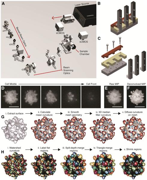
Figure 7
meSPIM Design and Bleb Segmentation Workflow
(A) Detailed rendering of the meSPIM optical train (its components are described in detail in the microscope components folder within the meSPim Supplemental Information zip file ). (B and C) Mold for...
Figure images are served from the NIH/NLM PubMed Central Open Access Subset or Europe PMC; copyright remains with the publishers and authors.
💬 Discussion
0 commentsNo comments yet. Be the first to start a discussion!
Leave a Comment