Abstract
AbstractAs x-ray and electron tomography is pushed further into the nanoscale, the limitations of rotation stages become more apparent, leading to challenges in the alignment of the acquired projection images. Here we present an approach for rapid post-acquisition alignment of these projections to obtain high quality three-dimensional images. Our approach is based on a joint estimation of alignment errors, and the object, using an iterative refinement procedure. With simulated data where we know the alignment error of each projection image, our approach shows a residual alignment error that is a factor of a thousand smaller, and it reaches the same error level in the reconstructed image in less than half the number of iterations. We then show its application to experimental data in x-ray and electron nanotomography.
🔬 Techniques
💻 Software
🧪 Sample Preparation
🏭 Microscope Brands
📷 Detectors
💻 Software Details
💻 Code & Software
💾 Data Repositories
🏛️ Research Organizations (ROR)
Affiliated research institutions:
📋 Methods
Experimental validation
Having characterized the performance improvements of our joint iterative reconstruction approach (Algorithm 2) on simulated data, we then used it to obtain object slice reconstructions from the four experimental datasets: three from various x-ray microscopes, and one from an electron microscope. Sinograms and reconstructed object slices are shown in Fig. 9 both before and after the application of our joint iterative reprojection approach for compensating alignment errors. The severity of the alignment errors in each of the nanotomography datasets can be seen in by the “wiggles” in the unaligned sinograms as compared to the aligned sinograms, and the improvement in reconstructed image quality is evident. Figure 9 Sinograms, and reconstructed object slices, for the four different experimental datasets described in the Methods section (XRF = x-ray fluorescence, TXM = transmission x-ray microscopy, and EM = electron microscopy). The severity of the alignment errors in these tomographic datasets can be seen from the “wiggles” in the unaligned sinograms, and the poor quality of the reconstructed images. Our joint iterative reprojection reconstruction method provides the alignment information to remove these “wiggles” in the sinograms, and the reconstructed images are of much higher quality. Figure 10 shows the convergence rates of transverse (blue) and axial (red) alignment parameters using the experimental Dataset B. The axial alignment convergence was faster than in the transverse direction; however, both converged after about 50 iterations. The convergence rates are similar to those we observed in simulation studies as shown in Fig. 5 . Figure 10 Convergence plots of the joint (Algorithm 2) iterative reprojection approach as applied to Dataset B, one of the experimental datasets. The blue and red curve show the relative mean squared error (MSE) for each successive iteration of the algorithm for transverse and axial alignments, respectively.
Show full methods section
Experimental validation
Having characterized the performance improvements of our joint iterative reconstruction approach (Algorithm 2) on simulated data, we then used it to obtain object slice reconstructions from the four experimental datasets: three from various x-ray microscopes, and one from an electron microscope. Sinograms and reconstructed object slices are shown in Fig. 9 both before and after the application of our joint iterative reprojection approach for compensating alignment errors. The severity of the alignment errors in each of the nanotomography datasets can be seen in by the “wiggles” in the unaligned sinograms as compared to the aligned sinograms, and the improvement in reconstructed image quality is evident. Figure 9 Sinograms, and reconstructed object slices, for the four different experimental datasets described in the Methods section (XRF = x-ray fluorescence, TXM = transmission x-ray microscopy, and EM = electron microscopy). The severity of the alignment errors in these tomographic datasets can be seen from the “wiggles” in the unaligned sinograms, and the poor quality of the reconstructed images. Our joint iterative reprojection reconstruction method provides the alignment information to remove these “wiggles” in the sinograms, and the reconstructed images are of much higher quality. Figure 10 shows the convergence rates of transverse (blue) and axial (red) alignment parameters using the experimental Dataset B. The axial alignment convergence was faster than in the transverse direction; however, both converged after about 50 iterations. The convergence rates are similar to those we observed in simulation studies as shown in Fig. 5 . Figure 10 Convergence plots of the joint (Algorithm 2) iterative reprojection approach as applied to Dataset B, one of the experimental datasets. The blue and red curve show the relative mean squared error (MSE) for each successive iteration of the algorithm for transverse and axial alignments, respectively.
Methods Problem definition
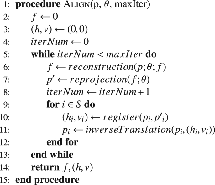
Here, we describe the mathematical basis of the alignment problem for 3D tomography. Let documentclass[12pt]{minimal} usepackage{amsmath} usepackage{wasysym} usepackage{amsfonts} usepackage{amssymb} usepackage{amsbsy} usepackage{mathrsfs} usepackage{upgreek} setlength{oddsidemargin}{-69pt} begin{document}$$f(x,y,z)$$end{document} f ( x , y , z ) be an unknown 3D object to be recovered. This can be expressed as a vector documentclass[12pt]{minimal} usepackage{amsmath} usepackage{wasysym} usepackage{amsfonts} usepackage{amssymb} usepackage{amsbsy} usepackage{mathrsfs} usepackage{upgreek} setlength{oddsidemargin}{-69pt} begin{document}$$f=[{f}_{1},{f}_{2},ldots ,{f}_{N}{]}^{T}$$end{document} f = [ f 1 , f 2 , … , f N ] T , where documentclass[12pt]{minimal} usepackage{amsmath} usepackage{wasysym} usepackage{amsfonts} usepackage{amssymb} usepackage{amsbsy} usepackage{mathrsfs} usepackage{upgreek} setlength{oddsidemargin}{-69pt} begin{document}$$N={N}_{1}times {N}_{2}times {N}_{3}$$end{document} N = N 1 × N 2 × N 3 is the total number of voxels in documentclass[12pt]{minimal} usepackage{amsmath} usepackage{wasysym} usepackage{amsfonts} usepackage{amssymb} usepackage{amsbsy} usepackage{mathrsfs} usepackage{upgreek} setlength{oddsidemargin}{-69pt} begin{document}$$f$$end{document} f . Let the vector documentclass[12pt]{minimal} usepackage{amsmath} usepackage{wasysym} usepackage{amsfonts} usepackage{amssymb} usepackage{amsbsy} usepackage{mathrsfs} usepackage{upgreek} setlength{oddsidemargin}{-69pt} begin{document}$${p}_{i}$$end{document} p i represents a 2D projection image with documentclass[12pt]{minimal} usepackage{amsmath} usepackage{wasysym} usepackage{amsfonts} usepackage{amssymb} usepackage{amsbsy} usepackage{mathrsfs} usepackage{upgreek} setlength{oddsidemargin}{-69pt} begin{document}$$M={M}_{1}times {M}_{2}$$end{document} M = M 1 × M 2 pixels captured at the documentclass[12pt]{minimal} usepackage{amsmath} usepackage{wasysym} usepackage{amsfonts} usepackage{amssymb} usepackage{amsbsy} usepackage{mathrsfs} usepackage{upgreek} setlength{oddsidemargin}{-69pt} begin{document}$${i}^{th}$$end{document} i t h tilt angle documentclass[12pt]{minimal} usepackage{amsmath} usepackage{wasysym} usepackage{amsfonts} usepackage{amssymb} usepackage{amsbsy} usepackage{mathrsfs} usepackage{upgreek} setlength{oddsidemargin}{-69pt} begin{document}$${theta }_{i}$$end{document} θ i . Ideally (without any translation error), the measurement process for each projection can be represented by, 1 documentclass[12pt]{minimal} usepackage{amsmath} usepackage{wasysym} usepackage{amsfonts} usepackage{amssymb} usepackage{amsbsy} usepackage{mathrsfs} usepackage{upgreek} setlength{oddsidemargin}{-69pt} begin{document}$${p}_{i}={W}_{i}({theta }_{i})f+{e}_{i},quad i=mathrm{1,}ldots ,S,$$end{document} p i = W i ( θ i ) f + e i , i = 1, … , S , where documentclass[12pt]{minimal} usepackage{amsmath} usepackage{wasysym} usepackage{amsfonts} usepackage{amssymb} usepackage{amsbsy} usepackage{mathrsfs} usepackage{upgreek} setlength{oddsidemargin}{-69pt} begin{document}$${p}_{i}$$end{document} p i and documentclass[12pt]{minimal} usepackage{amsmath} usepackage{wasysym} usepackage{amsfonts} usepackage{amssymb} usepackage{amsbsy} usepackage{mathrsfs} usepackage{upgreek} setlength{oddsidemargin}{-69pt} begin{document}$${W}_{i}({theta }_{i})$$end{document} W i ( θ i ) are, respectively, the recorded projection data and the projection matrices for the documentclass[12pt]{minimal} usepackage{amsmath} usepackage{wasysym} usepackage{amsfonts} usepackage{amssymb} usepackage{amsbsy} usepackage{mathrsfs} usepackage{upgreek} setlength{oddsidemargin}{-69pt} begin{document}$${i}^{th}$$end{document} i t h tilt angle, and documentclass[12pt]{minimal} usepackage{amsmath} usepackage{wasysym} usepackage{amsfonts} usepackage{amssymb} usepackage{amsbsy} usepackage{mathrsfs} usepackage{upgreek} setlength{oddsidemargin}{-69pt} begin{document}$$e$$end{document} e is the additive measurement noise during the acquisition process. Now we consider the translation model. The 3D object f can freely translate in the documentclass[12pt]{minimal} usepackage{amsmath} usepackage{wasysym} usepackage{amsfonts} usepackage{amssymb} usepackage{amsbsy} usepackage{mathrsfs} usepackage{upgreek} setlength{oddsidemargin}{-69pt} begin{document}$$x$$end{document} x , documentclass[12pt]{minimal} usepackage{amsmath} usepackage{wasysym} usepackage{amsfonts} usepackage{amssymb} usepackage{amsbsy} usepackage{mathrsfs} usepackage{upgreek} setlength{oddsidemargin}{-69pt} begin{document}$$y$$end{document} y , and documentclass[12pt]{minimal} usepackage{amsmath} usepackage{wasysym} usepackage{amsfonts} usepackage{amssymb} usepackage{amsbsy} usepackage{mathrsfs} usepackage{upgreek} setlength{oddsidemargin}{-69pt} begin{document}$$z$$end{document} z directions, which leads to a 2D translation error over the projection images. Therefore, in our model, we apply the translation error to the 2D projection images instead of the 3D object (translation errors in the documentclass[12pt]{minimal} usepackage{amsmath} usepackage{wasysym} usepackage{amsfonts} usepackage{amssymb} usepackage{amsbsy} usepackage{mathrsfs} usepackage{upgreek} setlength{oddsidemargin}{-69pt} begin{document}$$z$$end{document} z direction have no effect in standard parallel-beam tomography). The measurement geometry and translations are given in Fig. 1 . The documentclass[12pt]{minimal} usepackage{amsmath} usepackage{wasysym} usepackage{amsfonts} usepackage{amssymb} usepackage{amsbsy} usepackage{mathrsfs} usepackage{upgreek} setlength{oddsidemargin}{-69pt} begin{document}$${i}^{th}$$end{document} i t h projection image can be described as documentclass[12pt]{minimal} usepackage{amsmath} usepackage{wasysym} usepackage{amsfonts} usepackage{amssymb} usepackage{amsbsy} usepackage{mathrsfs} usepackage{upgreek} setlength{oddsidemargin}{-69pt} begin{document}$${p}_{i}={T}_{i}({h}_{i},{v}_{i})W({theta }_{i})f$$end{document} p i = T i ( h i , v i ) W ( θ i ) f , where documentclass[12pt]{minimal} usepackage{amsmath} usepackage{wasysym} usepackage{amsfonts} usepackage{amssymb} usepackage{amsbsy} usepackage{mathrsfs} usepackage{upgreek} setlength{oddsidemargin}{-69pt} begin{document}$${T}_{i}$$end{document} T i represents an documentclass[12pt]{minimal} usepackage{amsmath} usepackage{wasysym} usepackage{amsfonts} usepackage{amssymb} usepackage{amsbsy} usepackage{mathrsfs} usepackage{upgreek} setlength{oddsidemargin}{-69pt} begin{document}$$Mtimes M$$end{document} M × M geometrical transformation operator, and documentclass[12pt]{minimal} usepackage{amsmath} usepackage{wasysym} usepackage{amsfonts} usepackage{amssymb} usepackage{amsbsy} usepackage{mathrsfs} usepackage{upgreek} setlength{oddsidemargin}{-69pt} begin{document}$${h}_{i},{v}_{i}$$end{document} h i , v i are unknown transverse and axial translation errors for documentclass[12pt]{minimal} usepackage{amsmath} usepackage{wasysym} usepackage{amsfonts} usepackage{amssymb} usepackage{amsbsy} usepackage{mathrsfs} usepackage{upgreek} setlength{oddsidemargin}{-69pt} begin{document}$${i}^{th}$$end{document} i t h projection image, respectively. If we stack the documentclass[12pt]{minimal} usepackage{amsmath} usepackage{wasysym} usepackage{amsfonts} usepackage{amssymb} usepackage{amsbsy} usepackage{mathrsfs} usepackage{upgreek} setlength{oddsidemargin}{-69pt} begin{document}$$S$$end{document} S projection images, Eqn. ( 1 ) can be rewritten in a compact form as, 2 documentclass[12pt]{minimal} usepackage{amsmath} usepackage{wasysym} usepackage{amsfonts} usepackage{amssymb} usepackage{amsbsy} usepackage{mathrsfs} usepackage{upgreek} setlength{oddsidemargin}{-69pt} begin{document}$$p=T(h,v)W(theta )f+e,$$end{document} p = T ( h , v ) W ( θ ) f + e , where documentclass[12pt]{minimal} usepackage{amsmath} usepackage{wasysym} usepackage{amsfonts} usepackage{amssymb} usepackage{amsbsy} usepackage{mathrsfs} usepackage{upgreek} setlength{oddsidemargin}{-69pt} begin{document}$$p=[{p}_{1},{p}_{2},ldots ,{p}_{S}{]}^{T}$$end{document} p = [ p 1 , p 2 , … , p S ] T is the vector of size documentclass[12pt]{minimal} usepackage{amsmath} usepackage{wasysym} usepackage{amsfonts} usepackage{amssymb} usepackage{amsbsy} usepackage{mathrsfs} usepackage{upgreek} setlength{oddsidemargin}{-69pt} begin{document}$$MStimes 1$$end{document} M S × 1 , holding the tomographic measurement dataset, documentclass[12pt]{minimal} usepackage{amsmath} usepackage{wasysym} usepackage{amsfonts} usepackage{amssymb} usepackage{amsbsy} usepackage{mathrsfs} usepackage{upgreek} setlength{oddsidemargin}{-69pt} begin{document}$$T(h,v)={rm{diag}}[{T}_{1}({h}_{1},{v}_{1}),{T}_{2}({h}_{2},{v}_{2}),ldots ,{T}_{S}({h}_{S},{v}_{S})]$$end{document} T ( h , v ) = diag [ T 1 ( h 1 , v 1 ) , T 2 ( h 2 , v 2 ) , … , T S ( h S , v S ) ] is the geometrical translation matrix of size documentclass[12pt]{minimal} usepackage{amsmath} usepackage{wasysym} usepackage{amsfonts} usepackage{amssymb} usepackage{amsbsy} usepackage{mathrsfs} usepackage{upgreek} setlength{oddsidemargin}{-69pt} begin{document}$$MStimes MS$$end{document} M S × M S , and documentclass[12pt]{minimal} usepackage{amsmath} usepackage{wasysym} usepackage{amsfonts} usepackage{amssymb} usepackage{amsbsy} usepackage{mathrsfs} usepackage{upgreek} setlength{oddsidemargin}{-69pt} begin{document}$$W(theta )=[{W}_{1}({theta }_{1}),{W}_{2}({theta }_{2}),ldots ,{W}_{S}({theta }_{S}{)]}^{T}$$end{document} W ( θ ) = [ W 1 ( θ 1 ) , W 2 ( θ 2 ) , … , W S ( θ S ) ] T is the matrix of size documentclass[12pt]{minimal} usepackage{amsmath} usepackage{wasysym} usepackage{amsfonts} usepackage{amssymb} usepackage{amsbsy} usepackage{mathrsfs} usepackage{upgreek} setlength{oddsidemargin}{-69pt} begin{document}$$MStimes N$$end{document} M S × N for the measurement process. Here documentclass[12pt]{minimal} usepackage{amsmath} usepackage{wasysym} usepackage{amsfonts} usepackage{amssymb} usepackage{amsbsy} usepackage{mathrsfs} usepackage{upgreek} setlength{oddsidemargin}{-69pt} begin{document}$$h=[{h}_{1},{h}_{2},ldots ,{h}_{S}{]}^{T}$$end{document} h = [ h 1 , h 2 , … , h S ] T and documentclass[12pt]{minimal} usepackage{amsmath} usepackage{wasysym} usepackage{amsfonts} usepackage{amssymb} usepackage{amsbsy} usepackage{mathrsfs} usepackage{upgreek} setlength{oddsidemargin}{-69pt} begin{document}$$v=[{v}_{1},{v}_{2},ldots ,{v}_{S}{]}^{T}$$end{document} v = [ v 1 , v 2 , … , v S ] T are unknown transverse and axial translation errors for all documentclass[12pt]{minimal} usepackage{amsmath} usepackage{wasysym} usepackage{amsfonts} usepackage{amssymb} usepackage{amsbsy} usepackage{mathrsfs} usepackage{upgreek} setlength{oddsidemargin}{-69pt} begin{document}$$S$$end{document} S projection images respectively, and documentclass[12pt]{minimal} usepackage{amsmath} usepackage{wasysym} usepackage{amsfonts} usepackage{amssymb} usepackage{amsbsy} usepackage{mathrsfs} usepackage{upgreek} setlength{oddsidemargin}{-69pt} begin{document}$$theta =[{theta }_{1},{theta }_{2},ldots ,{theta }_{S}{]}^{T}$$end{document} θ = [ θ 1 , θ 2 , … , θ S ] T denotes documentclass[12pt]{minimal} usepackage{amsmath} usepackage{wasysym} usepackage{amsfonts} usepackage{amssymb} usepackage{amsbsy} usepackage{mathrsfs} usepackage{upgreek} setlength{oddsidemargin}{-69pt} begin{document}$$S$$end{document} S tilt angles during the acquisition process. Algorithm 1 Proposed 3D joint alignment and reconstruction. The goal in the iterative reprojection tomography reconstruction is to recover both the translation error documentclass[12pt]{minimal} usepackage{amsmath} usepackage{wasysym} usepackage{amsfonts} usepackage{amssymb} usepackage{amsbsy} usepackage{mathrsfs} usepackage{upgreek} setlength{oddsidemargin}{-69pt} begin{document}$$(h,v)=({h}_{1},{v}_{1};{h}_{2},{v}_{2};ldots ;{h}_{S},{v}_{S})$$end{document} ( h , v ) = ( h 1 , v 1 ; h 2 , v 2 ; … ; h S , v S ) and the 3D object documentclass[12pt]{minimal} usepackage{amsmath} usepackage{wasysym} usepackage{amsfonts} usepackage{amssymb} usepackage{amsbsy} usepackage{mathrsfs} usepackage{upgreek} setlength{oddsidemargin}{-69pt} begin{document}$$f$$end{document} f simultaneously in a joint fashion. The most common way to achieve this is to minimize the distance between the real captured projection data and reprojection data calculated from the current reconstruction. Algorithm 11 summarizes the details of the proposed method. Implementation details We implemented our new approach (Algorithm 11) in Python while drawing upon openly available libraries. We used the open-source and documented package TomoPy 67 for the reconstruction and reprojection operators, and the open-source Scikit-Image library 68 for calculating phase-correlation based sub-pixel image registration 69 and image warping operators. The analytical phantoms and corresponding simulated measurements were generated using Xdesign 70 , which is another open-source Python package for simulating x-ray data.
Experimental datasets Dataset
A is of X-ray fluorescence data collected at the Bionanoprobe (BNP) 71 at the Advanced Photon Source at Argonne National Laboratory. This instrument uses a double crystal Si 111 monochromator to produce 10 keV incident x-rays, and a Fresnel zone plate to produce a focus spot with a theoretical Rayleigh resolution of 85 nm. A silicon drift detector was placed at 90° with regards to the incident X-ray beam direction to collect fluorescence signals from which element-specific images were obtained using the analysis program MAPS 72 . A tomographic dataset was obtained using projection images of 79 × 56 pixels at 60 nm pixel size and a dwell time of 100 msec per pixel, over a rotation angle range of 0° to 135° at 3° increments (0° refers to the sample plane being perpendicular to the incident X-ray beam). This dataset represents the X-ray fluorescence from a cluster of dried bacterial cells with a metallic surface tag imaged at room temperature; the maximum signal was about 50 detected photons per second.
Dataset
B is of Gadolinium x-ray fluorescence data collected at the Hard X-ray Nanoprobe (HXN) Beamline 73 , 74 at the National Synchrotron Light Source II (NSLS-II) of Brookhaven National Laboratory. As with the Bionanoprobe, a 10 keV beam was monochromatized, a Fresnel zone plate was used to produce a focus spot with a theoretical Rayleigh resolution of 49 nm, and a three-element fluorescence detector was placed at 90° to the incident beam to collect fluorescence signals from which element-specific images were obtained using PyXRF ( https://github.com/NSLS-II/PyXRF ), which is an equivalent elemental mapping software such as MAPS. A tomographic dataset was obtained using projection images of documentclass[12pt]{minimal} usepackage{amsmath} usepackage{wasysym} usepackage{amsfonts} usepackage{amssymb} usepackage{amsbsy} usepackage{mathrsfs} usepackage{upgreek} setlength{oddsidemargin}{-69pt} begin{document}$$200times 120$$end{document} 200 × 120 pixels at 25 nm pixel size and a dwell time of 30 msec per pixel (with a maximum Gd signal of about 450 detected photons per pixel), over a rotation angle range of −90° to +90° at 3° increments. The sample used was a ceramic composite with mixed ionic and electronic conductivity 75 , consisting of a Ce 0.8 Gd0.2O 2 (CGO) oxygen ionic conductive phase and a CoFe 2 O 4 (CFO) electronic conductive phase. Nanostructure at the grain boundary is expected to have significant impact on the conductivity of this material 75 .
Dataset
C is of 8 keV x-ray transmission data collected at the Transmission X-ray Microscope (TXM) of sector 32-ID at the Advanced Photon Source 76 . This microscope uses a specialized diffractive condenser optic to illuminate the sample, and a Fresnel zone plate objective with an experimentally measured resolution of 60 nm to produce a magnified image on a scintillator/lens/CCD image detector system. A tomographic dataset was obtained using projection images of documentclass[12pt]{minimal} usepackage{amsmath} usepackage{wasysym} usepackage{amsfonts} usepackage{amssymb} usepackage{amsbsy} usepackage{mathrsfs} usepackage{upgreek} setlength{oddsidemargin}{-69pt} begin{document}$$2160times 2560$$end{document} 2160 × 2560 pixels each at 15 nm pixel size and a per-projection acquisition time of 1 second, over a rotation angle range of −90° to +90° at 0.25° increments. The dataset was then downsampled documentclass[12pt]{minimal} usepackage{amsmath} usepackage{wasysym} usepackage{amsfonts} usepackage{amssymb} usepackage{amsbsy} usepackage{mathrsfs} usepackage{upgreek} setlength{oddsidemargin}{-69pt} begin{document}$$4times $$end{document} 4 × to documentclass[12pt]{minimal} usepackage{amsmath} usepackage{wasysym} usepackage{amsfonts} usepackage{amssymb} usepackage{amsbsy} usepackage{mathrsfs} usepackage{upgreek} setlength{oddsidemargin}{-69pt} begin{document}$$540times 640$$end{document} 540 × 640 pixels, from which a documentclass[12pt]{minimal} usepackage{amsmath} usepackage{wasysym} usepackage{amsfonts} usepackage{amssymb} usepackage{amsbsy} usepackage{mathrsfs} usepackage{upgreek} setlength{oddsidemargin}{-69pt} begin{document}$$200times 200$$end{document} 200 × 200 pixel subregion was extracted at each projection angle for tomographic reconstruction. The 32-ID TZXM is equipped with an air bearing rotation stage with documentclass[12pt]{minimal} usepackage{amsmath} usepackage{wasysym} usepackage{amsfonts} usepackage{amssymb} usepackage{amsbsy} usepackage{mathrsfs} usepackage{upgreek} setlength{oddsidemargin}{-69pt} begin{document}$$ sim 1.25$$end{document} ~ 1.25 documentclass[12pt]{minimal} usepackage{amsmath} usepackage{wasysym} usepackage{amsfonts} usepackage{amssymb} usepackage{amsbsy} usepackage{mathrsfs} usepackage{upgreek} setlength{oddsidemargin}{-69pt} begin{document}$$mu $$end{document} μ rad wobble and an eccentricity of documentclass[12pt]{minimal} usepackage{amsmath} usepackage{wasysym} usepackage{amsfonts} usepackage{amssymb} usepackage{amsbsy} usepackage{mathrsfs} usepackage{upgreek} setlength{oddsidemargin}{-69pt} begin{document}$$pm 100$$end{document} ± 100 nm over 360°, so this dataset had fewer initial alignment errors than the x-ray fluorescence datasets A and B though thermal drifts can still affect specimen translation over the 20 minute data acquisition time. The sample used was a cathode particle agglomerate (Li 1.2 Co 0.1 Ni 0.15 Mn 0.55 O 2 ) of a Lithium-ion battery with volume of about 6 documentclass[12pt]{minimal} usepackage{amsmath} usepackage{wasysym} usepackage{amsfonts} usepackage{amssymb} usepackage{amsbsy} usepackage{mathrsfs} usepackage{upgreek} setlength{oddsidemargin}{-69pt} begin{document}$$mu m{}^{3}$$end{document} μ m 3 .
Dataset
D is of 200 kV high-angle annular dark field (HAADF) data acquired using a Hitachi HD2300 scanning transmission electron microscope at the Northwestern University Atomic and Nanoscale Characterization Experimental Center (NU ANCE ). A tomographic dataset was obtained using projection images of 256 × 256 pixels at 66 nm pixel size and a per-pixel dwell time of 10 documentclass[12pt]{minimal} usepackage{amsmath} usepackage{wasysym} usepackage{amsfonts} usepackage{amssymb} usepackage{amsbsy} usepackage{mathrsfs} usepackage{upgreek} setlength{oddsidemargin}{-69pt} begin{document}$$mu $$end{document} μ sec, over a rotation angle range of −60° to +60° at 1° increments. A nano-diffraction beam setting was used in order to maintain sufficient depth of focus. The specimen imaged was a human buccal cell collected utilizing a Cytobrush and deposited on a TEM grid. The sample was chemically fixed with glutaraldehyde (2.5%) and formaldehyde (2%) in PBS for 20 minutes. After fixation, the sample was gently washed and then plunge-frozen in liquid ethane (Vitrobot Mark III, FEI) and turbo freeze dried (K775X, Emitech). The dry sample was then plunge-frozen again, transferred to a cryo single tilt holder (Gatan) and kept at liquid nitrogen temperatures during imaging.
Data availability
The algorithms used here are made publicly available in the TomoPy package at https://tomopy.readthedocs.io . The simulated and experimental datasets used are available in TomoBank at https://tomobank.readthedocs.io .
Experimental datasets Dataset
A is of X-ray fluorescence data collected at the Bionanoprobe (BNP) 71 at the Advanced Photon Source at Argonne National Laboratory. This instrument uses a double crystal Si 111 monochromator to produce 10 keV incident x-rays, and a Fresnel zone plate to produce a focus spot with a theoretical Rayleigh resolution of 85 nm. A silicon drift detector was placed at 90° with regards to the incident X-ray beam direction to collect fluorescence signals from which element-specific images were obtained using the analysis program MAPS 72 . A tomographic dataset was obtained using projection images of 79 × 56 pixels at 60 nm pixel size and a dwell time of 100 msec per pixel, over a rotation angle range of 0° to 135° at 3° increments (0° refers to the sample plane being perpendicular to the incident X-ray beam). This dataset represents the X-ray fluorescence from a cluster of dried bacterial cells with a metallic surface tag imaged at room temperature; the maximum signal was about 50 detected photons per second.
Dataset
B is of Gadolinium x-ray fluorescence data collected at the Hard X-ray Nanoprobe (HXN) Beamline 73 , 74 at the National Synchrotron Light Source II (NSLS-II) of Brookhaven National Laboratory. As with the Bionanoprobe, a 10 keV beam was monochromatized, a Fresnel zone plate was used to produce a focus spot with a theoretical Rayleigh resolution of 49 nm, and a three-element fluorescence detector was placed at 90° to the incident beam to collect fluorescence signals from which element-specific images were obtained using PyXRF ( https://github.com/NSLS-II/PyXRF ), which is an equivalent elemental mapping software such as MAPS. A tomographic dataset was obtained using projection images of documentclass[12pt]{minimal} usepackage{amsmath} usepackage{wasysym} usepackage{amsfonts} usepackage{amssymb} usepackage{amsbsy} usepackage{mathrsfs} usepackage{upgreek} setlength{oddsidemargin}{-69pt} begin{document}$$200times 120$$end{document} 200 × 120 pixels at 25 nm pixel size and a dwell time of 30 msec per pixel (with a maximum Gd signal of about 450 detected photons per pixel), over a rotation angle range of −90° to +90° at 3° increments. The sample used was a ceramic composite with mixed ionic and electronic conductivity 75 , consisting of a Ce 0.8 Gd0.2O 2 (CGO) oxygen ionic conductive phase and a CoFe 2 O 4 (CFO) electronic conductive phase. Nanostructure at the grain boundary is expected to have significant impact on the conductivity of this material 75 .
Dataset
C is of 8 keV x-ray transmission data collected at the Transmission X-ray Microscope (TXM) of sector 32-ID at the Advanced Photon Source 76 . This microscope uses a specialized diffractive condenser optic to illuminate the sample, and a Fresnel zone plate objective with an experimentally measured resolution of 60 nm to produce a magnified image on a scintillator/lens/CCD image detector system. A tomographic dataset was obtained using projection images of documentclass[12pt]{minimal} usepackage{amsmath} usepackage{wasysym} usepackage{amsfonts} usepackage{amssymb} usepackage{amsbsy} usepackage{mathrsfs} usepackage{upgreek} setlength{oddsidemargin}{-69pt} begin{document}$$2160times 2560$$end{document} 2160 × 2560 pixels each at 15 nm pixel size and a per-projection acquisition time of 1 second, over a rotation angle range of −90° to +90° at 0.25° increments. The dataset was then downsampled documentclass[12pt]{minimal} usepackage{amsmath} usepackage{wasysym} usepackage{amsfonts} usepackage{amssymb} usepackage{amsbsy} usepackage{mathrsfs} usepackage{upgreek} setlength{oddsidemargin}{-69pt} begin{document}$$4times $$end{document} 4 × to documentclass[12pt]{minimal} usepackage{amsmath} usepackage{wasysym} usepackage{amsfonts} usepackage{amssymb} usepackage{amsbsy} usepackage{mathrsfs} usepackage{upgreek} setlength{oddsidemargin}{-69pt} begin{document}$$540times 640$$end{document} 540 × 640 pixels, from which a documentclass[12pt]{minimal} usepackage{amsmath} usepackage{wasysym} usepackage{amsfonts} usepackage{amssymb} usepackage{amsbsy} usepackage{mathrsfs} usepackage{upgreek} setlength{oddsidemargin}{-69pt} begin{document}$$200times 200$$end{document} 200 × 200 pixel subregion was extracted at each projection angle for tomographic reconstruction. The 32-ID TZXM is equipped with an air bearing rotation stage with documentclass[12pt]{minimal} usepackage{amsmath} usepackage{wasysym} usepackage{amsfonts} usepackage{amssymb} usepackage{amsbsy} usepackage{mathrsfs} usepackage{upgreek} setlength{oddsidemargin}{-69pt} begin{document}$$ sim 1.25$$end{document} ~ 1.25 documentclass[12pt]{minimal} usepackage{amsmath} usepackage{wasysym} usepackage{amsfonts} usepackage{amssymb} usepackage{amsbsy} usepackage{mathrsfs} usepackage{upgreek} setlength{oddsidemargin}{-69pt} begin{document}$$mu $$end{document} μ rad wobble and an eccentricity of documentclass[12pt]{minimal} usepackage{amsmath} usepackage{wasysym} usepackage{amsfonts} usepackage{amssymb} usepackage{amsbsy} usepackage{mathrsfs} usepackage{upgreek} setlength{oddsidemargin}{-69pt} begin{document}$$pm 100$$end{document} ± 100 nm over 360°, so this dataset had fewer initial alignment errors than the x-ray fluorescence datasets A and B though thermal drifts can still affect specimen translation over the 20 minute data acquisition time. The sample used was a cathode particle agglomerate (Li 1.2 Co 0.1 Ni 0.15 Mn 0.55 O 2 ) of a Lithium-ion battery with volume of about 6 documentclass[12pt]{minimal} usepackage{amsmath} usepackage{wasysym} usepackage{amsfonts} usepackage{amssymb} usepackage{amsbsy} usepackage{mathrsfs} usepackage{upgreek} setlength{oddsidemargin}{-69pt} begin{document}$$mu m{}^{3}$$end{document} μ m 3 .
Dataset
D is of 200 kV high-angle annular dark field (HAADF) data acquired using a Hitachi HD2300 scanning transmission electron microscope at the Northwestern University Atomic and Nanoscale Characterization Experimental Center (NU ANCE ). A tomographic dataset was obtained using projection images of 256 × 256 pixels at 66 nm pixel size and a per-pixel dwell time of 10 documentclass[12pt]{minimal} usepackage{amsmath} usepackage{wasysym} usepackage{amsfonts} usepackage{amssymb} usepackage{amsbsy} usepackage{mathrsfs} usepackage{upgreek} setlength{oddsidemargin}{-69pt} begin{document}$$mu $$end{document} μ sec, over a rotation angle range of −60° to +60° at 1° increments. A nano-diffraction beam setting was used in order to maintain sufficient depth of focus. The specimen imaged was a human buccal cell collected utilizing a Cytobrush and deposited on a TEM grid. The sample was chemically fixed with glutaraldehyde (2.5%) and formaldehyde (2%) in PBS for 20 minutes. After fixation, the sample was gently washed and then plunge-frozen in liquid ethane (Vitrobot Mark III, FEI) and turbo freeze dried (K775X, Emitech). The dry sample was then plunge-frozen again, transferred to a cryo single tilt holder (Gatan) and kept at liquid nitrogen temperatures during imaging.
📊 Figures
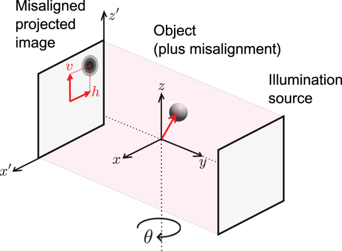
Figure 1
Schematic of the tomographic data acquisition process. Misalignment of the object in 3D space leads to a different 2D translation error ( h , v ) on each projection image taken at tilt angle u03b8 .
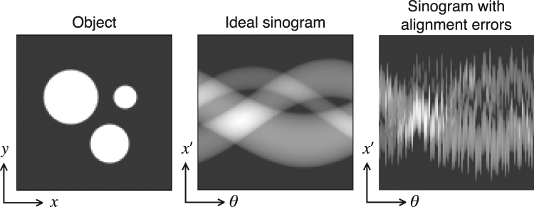
Figure 2
A transverse slice of the analytical 3D simulation phantom (left), ideal sinogram with no translation errors corresponding to the phantom (middle), and the sinogram after random shifts are applied (ri...
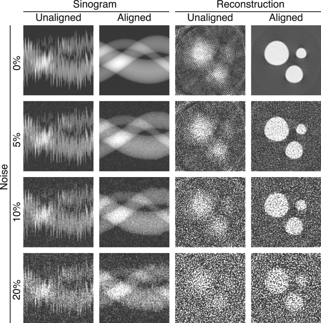
Figure 3
Joint reprojection/reconstruction results on the simulated 3D phantom shown in Fig. 2 . Alignment errors distributed uniformly over a range of u221210 to +10 pixels were applied to each projection, af...
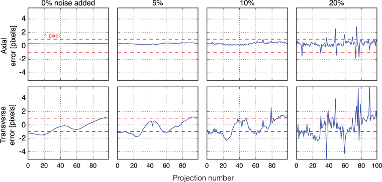
Figure 4
Estimation errors in image pixel units between true and recovered alignment parameters for both transverse (top row) and axial (bottom row) shifts and for different measurement noise levels. The estim...
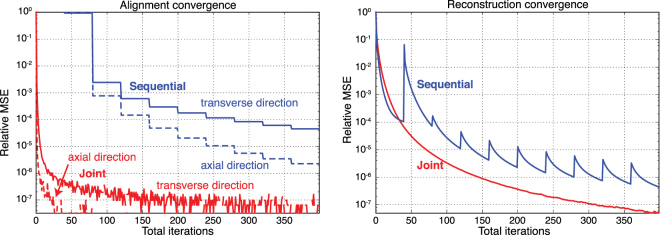
Figure 5
Convergence plots of the sequential (Algorithm 1) and our joint (Algorithm 2) iterative reprojection approach as applied to our simulated dataset of Fig. 2 . We show at left the mean square error (MSE...
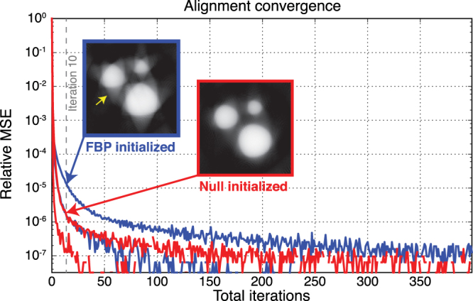
Figure 6
Convergence rates of joint alignment algorithm with different initializations. Blue and red plots corresponds to the relative mean squared error (MSE) in axial (rapidly convergent plot) and transverse...
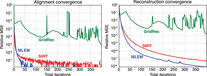
Figure 7
Comparison of three different reconstruction algorithms with respect to convergence rates for the alignment and object estimations with our joint algorithm as applied to our simulated dataset of Fig. ...
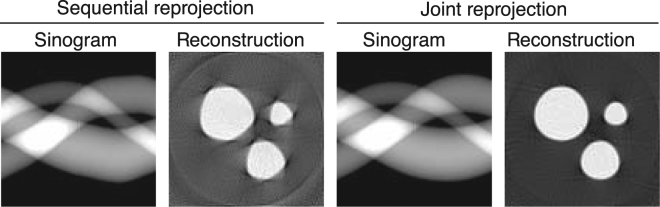
Figure 8
Reconstructed sinogram and corresponding tomographic reconstruction after the convergence of both the sequential (Algorithm 1) and joint (Algorithm 2) iterative reprojection approaches. As can be seen...
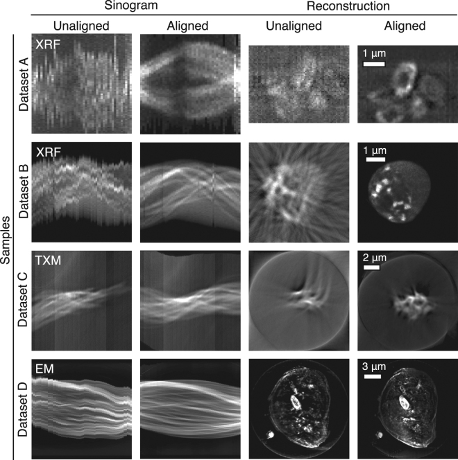
Figure 9
Sinograms, and reconstructed object slices, for the four different experimental datasets described in the Methods section (XRFu2009=u2009x-ray fluorescence, TXMu2009=u2009transmission x-ray microscopy...
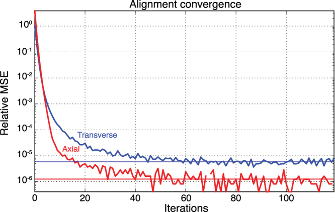
Figure 10
Convergence plots of the joint (Algorithm 2) iterative reprojection approach as applied to Dataset B, one of the experimental datasets. The blue and red curve show the relative mean squared error (MSE...
Algorithm 1
Proposed 3D joint alignment and reconstruction.
Figure images are served from the NIH/NLM PubMed Central Open Access Subset or Europe PMC; copyright remains with the publishers and authors.
💬 Discussion
0 commentsNo comments yet. Be the first to start a discussion!
Leave a Comment