Abstract
Maximal resection of tumor while preserving the adjacent healthy tissue is particularly important for larynx surgery, hence precise and rapid intraoperative histology of laryngeal tissue is crucial for providing optimal surgical outcomes. We hypothesized that deep-learning based stimulated Raman scattering (SRS) microscopy could provide automated and accurate diagnosis of laryngeal squamous cell carcinoma on fresh, unprocessed surgical specimens without fixation, sectioning or staining. Methods: We first compared 80 pairs of adjacent frozen sections imaged with SRS and standard hematoxylin and eosin histology to evaluate their concordance. We then applied SRS imaging on fresh surgical tissues from 45 patients to reveal key diagnostic features, based on which we have constructed a deep learning based model to generate automated histologic results. 18,750 SRS fields of views were used to train and cross-validate our 34-layered residual convolutional neural network, which was used to classify 33 untrained fresh larynx surgical samples into normal and neoplasia. Furthermore, we simulated intraoperative evaluation of resection margins on totally removed larynxes. Results: We demonstrated near-perfect diagnostic concordance (Cohen's kappa, κ > 0.90) between SRS and standard histology as evaluated by three pathologists. And deep-learning based SRS correctly classified 33 independent surgical specimens with 100% accuracy. We also demonstrated that our method could identify tissue neoplasia at the simulated resection margins that appear grossly normal with naked eyes. Conclusion: Our results indicated that SRS histology integrated with deep learning algorithm provides potential for delivering rapid intraoperative diagnosis that could aid the surgical management of laryngeal cancer.
🔬 Techniques
🔭 Microscopes
💻 Software
✨ Fluorophores
🧪 Sample Preparation
🏭 Microscope Brands
🧪 Reagent Suppliers
🔴 Lasers
📷 Detectors
🔎 Objectives
🎨 Filters
💻 Software Details
🏛️ Research Organizations (ROR)
Affiliated research institutions:
📋 Methods
Tissue collection and preparation
All tissue samples were collected from patients in Zhejiang Provincial People's Hospital, and approved by the Ethics Committee with informed written consent (KY2015260). Surgical tissues were removed following standard operative procedures. Laryngeal squamous cell carcinoma tissues were from clinical diagnosed biopsies, and normal tissues were largely taken from vocal cord polypus. To prepare frozen sections, surgical specimens were snap frozen in liquid nitrogen and stored at -80 0 C until sectioned with freezing microtome (CM 1950, Leica). Thin sections of 20 µm thicknesses were used for SRS imaging, and adjacent 5 µm thick sections were sent for H&E staining. All fresh samples and thin sections were maintained at low temperature with dry ice and delivered to Fudan University within 7 hours through express transportation. Fresh tissues were sliced manually with a razor blade and then sealed between two coverslips and a perforated glass slide (0.5 mm thick) for direct SRS imaging. Thin frozen tissue sections were simply covered with coverslips, and imaged without further processing. Totally removed larynxes were taken from patients of advanced laryngeal SCC for simulated surgeries and evaluations of resection margins. In total, 78 patient cases were involved in the database for imaging, model training and testing, more detailed information of all the cases are shown in Table S1 . For fresh tissues, 45 out of the 78 cases (21 normal and 24 cancerous) were used for model training and validation, whereas the residual 33 cases were kept untouched until the final testing. For frozen section analysis, 15 out of the 78 cases (marked in Table S1 ) were used to generate 80 pairs of adjacent sections for SRS and H&E imaging. For all these cases, standard H&E based histopathology were done on paraffin embedded sections and served as the “ground truth”.
Show full methods section
Tissue collection and preparation
All tissue samples were collected from patients in Zhejiang Provincial People's Hospital, and approved by the Ethics Committee with informed written consent (KY2015260). Surgical tissues were removed following standard operative procedures. Laryngeal squamous cell carcinoma tissues were from clinical diagnosed biopsies, and normal tissues were largely taken from vocal cord polypus. To prepare frozen sections, surgical specimens were snap frozen in liquid nitrogen and stored at -80 0 C until sectioned with freezing microtome (CM 1950, Leica). Thin sections of 20 µm thicknesses were used for SRS imaging, and adjacent 5 µm thick sections were sent for H&E staining. All fresh samples and thin sections were maintained at low temperature with dry ice and delivered to Fudan University within 7 hours through express transportation. Fresh tissues were sliced manually with a razor blade and then sealed between two coverslips and a perforated glass slide (0.5 mm thick) for direct SRS imaging. Thin frozen tissue sections were simply covered with coverslips, and imaged without further processing. Totally removed larynxes were taken from patients of advanced laryngeal SCC for simulated surgeries and evaluations of resection margins. In total, 78 patient cases were involved in the database for imaging, model training and testing, more detailed information of all the cases are shown in Table S1 . For fresh tissues, 45 out of the 78 cases (21 normal and 24 cancerous) were used for model training and validation, whereas the residual 33 cases were kept untouched until the final testing. For frozen section analysis, 15 out of the 78 cases (marked in Table S1 ) were used to generate 80 pairs of adjacent sections for SRS and H&E imaging. For all these cases, standard H&E based histopathology were done on paraffin embedded sections and served as the “ground truth”.
Microscope setup
The apparatus of our SRS based microscope is illustrated in Figure S1 . A commercial femtosecond (fs) optical parametric oscillator (OPO, Insight DS+, Newport) with dual outputs were used as the light source. The fundamental 1040 nm beam (~200 fs) was used as the Stokes, and the wavelength tunable output (690-1300 nm, ~ 150 fs) was used as the pump. Both beams were linearly chirped to several picoseconds (pump: ~ 3.8 ps, Stokes: ~ 1.8 ps) through highly dispersive SF57 glass rods to work in the “spectral focusing SRS” mode 17 , 44 , where the target Raman frequency could be adjusted by scanning the time delay between pump and Stokes pulses, instead of changing the wavelengths ( Figure S1 ). The Stokes beam was intensity modulated by an electro optical modulator (EOM) at 10 MHz, and collinearly combined with the pump beam through a dichroic mirror (DMSP1000, Thorlabs). The combined beam was delivered to the laser scanning microscope (FV1200, Olympus) and focused onto the samples with an objective (UPLSAPO 60XWIR, NA 1.2 water, Olympus). The transmitted stimulated Raman loss (SRL) signal of the pump beam was filtered with a band-pass filter (CARS ET890/220, Chroma), detected with a home-built back-biased photodiode and demodulated with a lock-in amplifier (HF2LI, Zurich Instruments) to generate pixel data for the microscope to form SRS images. In this study, we fixed the pump beam at 802 nm center wavelength, and imaged at two time delays which correspond to two Raman frequencies of 2845 cm -1 and 2930 cm -1 for lipid/protein decomposition. The SHG signal excited by the pump beam was simultaneously detected with a narrow band-pass filter (FF01-405/10-25, Semrock) and a photomultiplier (PMT) in the epi mode, generating images of collagen fiber distributions. The optical power of the pump and Stokes beams at the samples were kept at around 30 mW and 40 mW, respectively. Each field of view (FOV) was imaged with a size of 512 × 512 pixels and 2 µs pixel dwell time. Automated mosaic imaging method was applied to scan across large sample areas and all FOVs were stitched to form the full-sized images with custom written Matlab program. A typical 1 cm 2 tissue costs ~ 8 minutes to image under strip mosaicing mode 21 .
H&E staining
H&E staining was performed following the standard procedure. First, the tissue section was immersed in 100% methanol for 30 s and then stained in hematoxylin solution (Harris modified) for 1 minute. Sample was washed in deionized water for 10 seconds after each step. Next, we perform counterstain in 0.5% eosin solution for 60 s after dipping in bluing reagent [0.1% (v/v) ammonia water solution] for 1 s and washing in deionized water for 1 second. At last, we dipped the sample in xylene for 10 s twice after washing and dehydrating in 80%, 95% and 100% ethanol for 2 s, respectively. Dried Sections were sealed with neutral gum and a coverslip. All reagents used were purchased from Sigma-Aldrich. The final H&E slides were imaged on a home-built automated system, composed of a bright field microscope (IX73, Olympus), a CCD camera (MG 320 C Speed, Moogee) and a motorized XY stage (Tango, Marzhauser Wetzlar GmbH & Co.). Mosaic imaging and stitching were realized with custom softwares written in VB.net and Matlab.
Image processing Raw
SRS images taken at 2845 cm -1 and 2930 cm -1 need to be decomposed into lipids and proteins distributions. Because SRS signal is linearly proportional to chemical concentrations, we apply a simple linear algorithm for the decomposition with measured SRS spectra of standard lipid (oleic acid - OA) and protein (bovine serum albumin - BSA) as shown in Figure S1 and previous works 9 , 26 . We extracted protein (blue) signal by subtracting SRS signal at 2845 cm -1 from that of 2930 cm -1 , and the lipid (green) signal was directly taken from SRS signal at 2845 cm -1 . SHG data (red) was used without further processing. Because of the aberrations from object lens, signal intensity of each image FOV is not evenly distributed, usually brighter in the center. We used the intensity profile measured from a spatially homogeneous sample to correct/flatten each FOV, followed by our stitching program to merge all FOVs together.
Survey and statistical analysis
We collected survey results using a web-based survey tool (LimeSurvey), consisting of 80 pairs of SRS and H&E images from adjacent sister sections, which were mixed and shown in random order. Three blinded pathologists were briefly educated with the principle and image contrasts of SRS, then read the 160 images and categorized each image as “normal” or “neoplasia” based on the diagnostic features of either cytology or histoarchitecture. The rating results were based on the “ground truth” of standard histopathology on paraffin embedded sections. For each pathologist, survey responses were used to calculate Cohen's kappa statistic for normal versus neoplasia to determine concordance between SRS and H&E with statistical product and service solutions (SPSS) software 47 . We calculated the accuracies of the three pathologists using the ratio between the number of correct and total FOVs.
Deep-learning model
We constructed a ResNet34 model in Pytorch platform ( https://pytorch.org/ ). The model is a tensor and dynamic neural network written in python. In addition to 34 layers of plain convolutional neural network, ResNet34 contains identity mappings that allow the information of the input or gradient to pass through many layers. ResNet34 has 33 convolutional layers and 1 fully connected (fc) layer. The convolutional layers mostly capture the main local features of images with 3×3 filters, and the last fully connected layer gives a binary classification according to the global feature connected from all local features. It is worth noticing that batch normalization was employed in the same magnitude at each convolutional layer. To optimize the neural network, the weights of network were initialized randomly. Loss was calculated according to the cross entropy (log mean square error). The selected optimizer was the 'Adam' optimizer with the following parameters: lr =5×10 -5 , β 1 =0.9, β 2 =0.99, w =10 -4 ; where lr and w represent the learning rate and weight decay, respectively; β 1 and β 2 represent the memory lifetimes of the first and second moment 48 . Images were fed in batches with a batch size of 100. Data augmentation techniques were used to help produce similar but non-identical data, which could effectively enlarge image database for the training of deep-learning models 49 , 50 . In this work, we applied rotation, flipping and color jittering of images to effectively enlarge our image dataset. The random rotation angle was set to 20 degrees, and the probability of horizontal and vertical flipping is set to 0.5. The best color jitter values including image brightness, saturation and contrast fluctuations are set to 0.4.
Supplementary Material Supplementary figures and table; the optical setup; typical SRS and H&E images used for the survey; quantitative image analysis; and typical SRS images used for training deep-learning model. Click here for additional data file.
📊 Figures
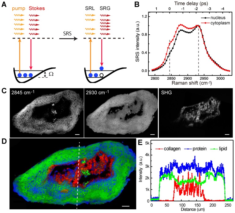
Figure 1
Experimental design. A, Illustration of stimulated Raman scattering process, which leads to the reduction of pump photons - stimulated Raman loss (SRL) and the gain of Stokes photons - stimulated Rama...
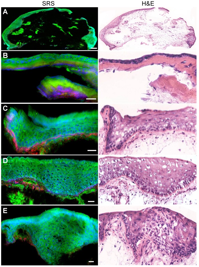
Figure 2
SRS and H&E images of adjacent frozen sections from normal laryngeal tissues. A, Typical large-scale images from normal laryngeal tissue. B-E, Zoom-in images demonstrating regular structures of the ba...
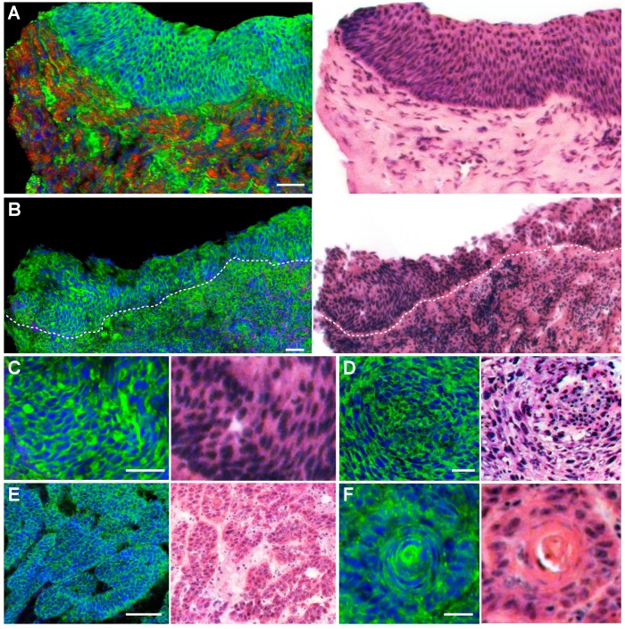
Figure 3
SRS and HE images of frozen sections from laryngeal squamous cell carcinoma tissues. A, Laryngeal SCC in situ. B, Invasive SCC. C, Cytological atypia. D, Cytological atypia accompanied with lymphocyte...
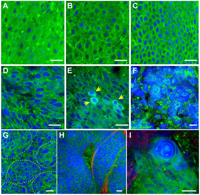
Figure 4
SRS imaging of unprocessed fresh larynx surgical tissues. A-C, Normal squamous cells imaged at various locations of the epithelium layer. Histological hallmarks of laryngeal SCC could be visualized, i...
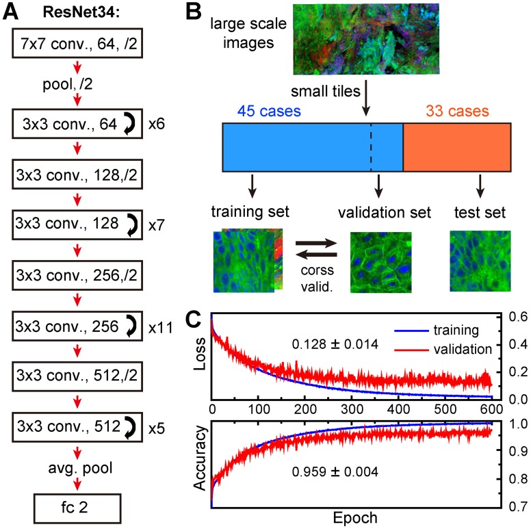
Figure 5
Construction and validation of deep-learning model. A, Network architecture of ResNet34. B, Schematic illustration of the work flow for training and validation of the model. C, Five-fold cross validat...
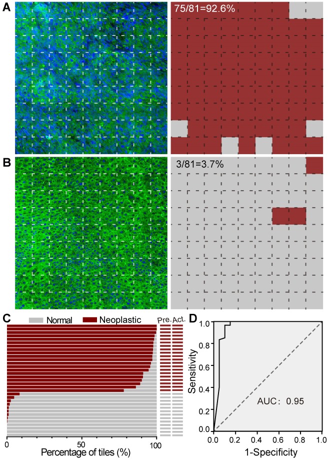
Figure 6
SRS histology of larynx tissue with the aid of ResNet34. A, Imaging and prediction results of a laryngeal SCC tissue. The large image was divided into small FOVs (77u00d777 u03bcm), and predictions we...
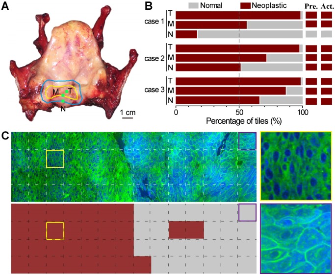
Figure 7
Evaluation of simulated resection margins with ResNet34-SRS. A, A typical totally removed larynx, showing the gross margin (yellow line) of the tumor and the estimated resection margin (blue line); ti...
Figure images are served from the NIH/NLM PubMed Central Open Access Subset or Europe PMC; copyright remains with the publishers and authors.
💬 Discussion
0 commentsNo comments yet. Be the first to start a discussion!
Leave a Comment