Abstract
Two-photon microscopy is widely used to investigate brain function across multiple spatial scales. However, measurements of neural activity are compromised by brain movement in behaving animals. Brain motion-induced artifacts are typically corrected using post hoc processing of two-dimensional images, but this approach is slow and does not correct for axial movements. Moreover, the deleterious effects of brain movement on high-speed imaging of small regions of interest and photostimulation cannot be corrected post hoc. To address this problem, we combined random-access three-dimensional (3D) laser scanning using an acousto-optic lens and rapid closed-loop field programmable gate array processing to track 3D brain movement and correct motion artifacts in real time at up to 1 kHz. Our recordings from synapses, dendrites and large neuronal populations in behaving mice and zebrafish demonstrate real-time movement-corrected 3D two-photon imaging with submicrometer precision.
🔬 Techniques
🧬 Organisms
✨ Fluorophores
🧪 Sample Preparation
🏭 Microscope Brands
🧪 Reagent Suppliers
🔴 Lasers
📷 Detectors
💻 Software Details
🏛️ Research Organizations (ROR)
Affiliated research institutions:
📋 Methods
Microscope and real-time 3D movement correction system The Acousto-Optic Lens (AOL) 3D two-photon microscope layout and real-time movement correction system is shown in Extended Data Figure 1 . Briefly, an 80 MHz pulsed Ti:Sapphire laser (Chameleon, Coherent, CA, USA) tuned to a wavelength of 920 nm was routed to the compact configuration AOL 28 via a custom designed prism-based pre-chirper (APE GmbH, Berlin), a Pockels cell (Model 302CE, Conoptics) and a custom made beam expander that increased the beam diameter to fill the 15 mm aperture of the AOL. The AOL consisted of two orthogonally arranged pairs of on-axis TeO 2 Acousto-optic deflectors (AODs Gooch and Housego) interleaved with quarter wave plates and polarisers to couple them together 4 , 28 . The AOL was controlled from an FPGA control board (Xilinx VC707) which had a custom designed, on-chip digital waveform synthesiser that generated radio frequency (RF) signals, which were passed to four digital-to-analog converters (DACs) at 275 MS s −1 (Two Texas Instruments DAC5672) and then amplified (PA-4 from InterAction Corp). Relay optics coupling the AOL to a customised SliceScope microscope (Scientifica, UK) were arranged to under-fill a 20X water immersion objective (Olympus XLUMPlanFLN, NA 1.0), giving an NA of ~0.6 on the illumination path, or overfill a 40X objective (Olympus LUMPlanFLN, NA 0.8). These objectives gave two-photon point spread functions with full width half maxima 0.69±0.04 μm (mean±SD) in XY and 6.54±0.27 μm in Z, and 0.58±0.03 μm in XY and 4.3±0.39 μm in Z, respectively, for 0.1 μm beads. Red and green channels were detected with GaAsP photomultiplier tubes (PMTs) (H7422, Hamamatsu, Japan) and digitised using high-speed 800 MSPS ADCs (NI-5772, National Instruments) via 200 MHz Pre-Amplifiers (Series DHPCA 100/200 MHz, FEMTO) and downsampled with a digital acquisition FPGA board (NI FlexRIO – 7966R, National Instruments) before sending frames to the host PC via the National Instruments PXIe interface. Custom 3D microscope interfaces written in MATLAB and LabVIEW environments and implemented on the host PC, were used to control the microscope and define imaging modes for Z stack acquisition, line scan and point-based functional imaging and motion correction. Imaging speed depends on the time required for the acoustic wave to propagate across the AOL aperture (fill time = 24.5 μs) and the dwell time per voxel (50 ns-13 μs). The fill time determines the time to jump from one location in the imaging volume to any other location and is required for each line scan or point measurement. Thus without Real-time 3D motion correction (RT-3DMC) the fastest frame time for imaging 512 line scans of 512 voxels each is 512x(24.5 + 512×0.05) = 25,651 μs or 39 Hz. Lower resolution images of the same FOV, or smaller FOVs, can be acquired much more rapidly (e.g. 256×256 voxels at 104 Hz) and point measurements can be performed at up to 40 kHz (i.e. 1/(24.5 + 0.5) = 0.04 MHz). RT-3DMC was achieved by periodically scanning a bead or soma located within the imaging volume, tracking its motion and adjusting the AOL 3D laser scanner to compensate for the motion ( Fig. 1c ). The acquisition FPGA contained a programmable timer that determined the feedback period for motion correction (typically, every 1–2 ms) and synchronised the AOL controller to correctly interleave reference scans with the main imaging sequence ( Extended Data Fig. 1 ). The RT-3DMC logic first scans a lateral XY reference image, calculates the XY offset and corrects the XY FOV prior to performing the Z-line scans. Pipelining this process per pixel reduced the time to perform the lateral update to 50–60 μs. Having centered the reference feature, Z line scans were performed to determine the axial position of the bead. The RT-3DMC logic contains a PID controller to optimise the current offset estimate (Δx, Δy, Δz) which are sent to the AOL controller via a serial link running the Serial Peripheral Interface (SPI) protocol. The SPI interface used a 16 bit field (±7 bits integer and 8 bits fractional), limiting the maximum tracking to ±128 reference pixels. The control FPGA converts the pixel offset to the acoustic frequency drives needed to track the brain motion in 3D, including compensating for any optical field distortions ( Supplementary Note 4 ). On-chip DSP blocks on the Xilinx Virtex 7 were used to calculate the movement corrected RF drive waveforms for each of the four AODs in parallel by executing fixed point-arithmetic operations at 125 MHz. Pre-fetching and calculating the four frequency offsets took 2x reference image frame size away). The experimental imaging procedure was as follows: RT-3DMC was set up by selecting a reference object for tracking, and an initial RT-3DMC Z-stack was acquired, from which the imaged structures (plane, subvolume, patches or points) were selected. All recordings with RT-3DMC were then done with this frame of reference. Following the RT-3DMC on sessions, the stage was manually realigned for the RT-3DMC off session to compensate for slow drift that had developed (RT-3DMC compensates for drift by adjusting the scans, without any stage movement). This allowed us to compare the same ROI across RT-3DMC on and off sessions. All mice were familiarised with the experimental setup and monitored to ensure they exhibited no signs of distress. During recordings, mice were free to stand or run on a cylindrical Styrofoam wheel. Locomotion was monitored with a rotary encoder and for experiments investigating brain movement during licking, a metal lick spout water dispenser was placed in front of the mouth. The water was enriched with 0.5 M sucrose. Running, licking and perioral motion were monitored with a video camera tracking at 50 Hz. The occurrence of perioral movement bouts were detected using a motion index (Motion Index = sum of the intensity difference between consecutive pixels values within the ROI) assay using ROIs drawn around the perioral region and among these, clear licking bouts were identified by visual inspection. For the longitudinal study we selected a 300×300×300–450 μm imaging volume in the motor cortex of each mouse. To precisely align the volume in XY we located a cell from the reference Z-stack taken on day 1, noted its pixel location, and moved the stage until it was precisely centred in the FOV. To align the volume in Z, we ensured the same bead used for tracking was 30 μm below the top of the Z-stack. We used the same PMT gain settings on the red and green channels, as well as laser power intensity per animal. To quantify changes in bead and tissue fluorescence, we collected RT-3DMC stabilised volumetric Z-stacks at the beginning and end of the imaging session. Longitudinal imaging sessions were 1–2 hrs per mouse per day. In vivo imaging in awake behaving zebrafish larvae. Zebrafish imaging: Tg(elavl3:H2B-GCaMP6s) 41 larvae carrying the mitfa− /− skin-pigmentation mutation were used for all experiments 42 . Larvae were raised in fish facility water at 28°C on a 14/10 h light/dark cycle and fed Paramecia from 4 days post fertilisation (dpf). All experimental procedures were approved by the UCL Animal Welfare Ethical Review Body and the UK Home Office under the Animal (Scientific Procedures) Act 1986. Injection of fluorescent beads: Larvae at 4 dpf were anaesthetised using MS222 (Sigma), and mounted upright in 3% low-melting point agarose (Sigma-Aldrich). A small piece of agarose was cut away with an ophthalmic scalpel to expose an area of the larvae’s head around the hindbrain ventricle. Yellow-green fluorescent beads with a diameter of 5 μm (Invitrogen) were suspended in Ringer’s solution (in mM: NaCl 123, CaCl 2 1.53, KCl 4.96 and pH 7.4), and injected into the hindbrain ventricle. Once the presence of fluorescent beads in the brain was confirmed, fish were unmounted from the agarose and left to recover. Where beads did not become securely embedded, fish were discarded as the bead tended to move during swims. Presentation of visual stimuli and behavioural tracking during two-photon microscopy: Larval zebrafish were partially restrained in agarose similar to ref. 43 . Larvae at 5–6 dpf were anaesthetised using MS222 and mounted upright in 3% agarose. Agarose around the eyes and tail were removed and the fish left to recover overnight before calcium imaging the following day. Visual stimuli consisted of optomotor gratings projected onto a diffusive screen below the fish using a sub-stage projector (AAXA P2 Jr Pico Projector). A Number 29 Wratten filter (Kodak) was placed in front of the projector to block green light from the PMT. Stimuli were designed using Psychophysics Toolbox 44 and moved in different directions (90°, 135°, 225°, 270° with respect to fish heading direction) at 1 cycle/s and with a period of 10 mm. A stimulus was presented every 30 s and drifted for 10 s. For behavioural tracking, the fish was illuminated by two 850 nm LEDs and imaged at 400 Hz by a sub-stage GS3-U3–41C6NIR-C camera (Point Grey). The tail was tracked online using machine vision algorithms 45 . Positive angles describe rightward tail bends, and negative angles describe leftward bends. Characterisation of brain motion and its relation to feedback time To quantify brain movement we imaged sparsely labelled somata in mouse primary motor cortex, visual cortex, cerebellar molecular layer at > 110 Hz during locomotion and licking and in zebrafish forebrain during swimming bouts. Tissue movement was quantified using post-hoc centroid analysis of selected cells and XY displacements, speed and frequency analysis were calculated using custom MATLAB scripts. Tuning the PID controller: We initially tuned the PID controller using a MATLAB simulation of the system using Z stack images from a mouse cortex with a feedback time of 2 ms. For this we used the Ziegler–Nichols method 46 to get initial values and then simulated oscillations with lateral RT-3DMC at frequencies from 1– 20 Hz and peak-to-peak amplitudes of 10–40 μm. An error metric was used to find the optimal value for P (0.8) and I (400) for 20 μm peak-to-peak amplitude oscillations at 1–20 Hz. We found that adding any differential term increased the feedback noise and caused instability, so we set D (0) for all experiments. We then reproduced the tuning on the microscope using 4-μm fluorescent beads and a piezo stage, and found these settings were optimal for up to 20 Hz and 20 μm peak-to-peak which is well within the range of mouse brain motion. Although these settings were optimal for sinusoidal oscillations, we found for the stochastic brain motion observed in animals (particularly zebrafish), that changing the proportional setting to P=0.9 was more robust and also worked well with mice. So for the vast majority of experiments reported in this paper, we used P=0.9, I = 400 and D = 0, for both mice and zebrafish. Supplementary Table 1 shows the parameters that can be adjusted to optimise motion correction.
Show full methods section
Microscope and real-time 3D movement correction system The Acousto-Optic Lens (AOL) 3D two-photon microscope layout and real-time movement correction system is shown in Extended Data Figure 1 . Briefly, an 80 MHz pulsed Ti:Sapphire laser (Chameleon, Coherent, CA, USA) tuned to a wavelength of 920 nm was routed to the compact configuration AOL 28 via a custom designed prism-based pre-chirper (APE GmbH, Berlin), a Pockels cell (Model 302CE, Conoptics) and a custom made beam expander that increased the beam diameter to fill the 15 mm aperture of the AOL. The AOL consisted of two orthogonally arranged pairs of on-axis TeO 2 Acousto-optic deflectors (AODs Gooch and Housego) interleaved with quarter wave plates and polarisers to couple them together 4 , 28 . The AOL was controlled from an FPGA control board (Xilinx VC707) which had a custom designed, on-chip digital waveform synthesiser that generated radio frequency (RF) signals, which were passed to four digital-to-analog converters (DACs) at 275 MS s −1 (Two Texas Instruments DAC5672) and then amplified (PA-4 from InterAction Corp). Relay optics coupling the AOL to a customised SliceScope microscope (Scientifica, UK) were arranged to under-fill a 20X water immersion objective (Olympus XLUMPlanFLN, NA 1.0), giving an NA of ~0.6 on the illumination path, or overfill a 40X objective (Olympus LUMPlanFLN, NA 0.8). These objectives gave two-photon point spread functions with full width half maxima 0.69±0.04 μm (mean±SD) in XY and 6.54±0.27 μm in Z, and 0.58±0.03 μm in XY and 4.3±0.39 μm in Z, respectively, for 0.1 μm beads. Red and green channels were detected with GaAsP photomultiplier tubes (PMTs) (H7422, Hamamatsu, Japan) and digitised using high-speed 800 MSPS ADCs (NI-5772, National Instruments) via 200 MHz Pre-Amplifiers (Series DHPCA 100/200 MHz, FEMTO) and downsampled with a digital acquisition FPGA board (NI FlexRIO – 7966R, National Instruments) before sending frames to the host PC via the National Instruments PXIe interface. Custom 3D microscope interfaces written in MATLAB and LabVIEW environments and implemented on the host PC, were used to control the microscope and define imaging modes for Z stack acquisition, line scan and point-based functional imaging and motion correction. Imaging speed depends on the time required for the acoustic wave to propagate across the AOL aperture (fill time = 24.5 μs) and the dwell time per voxel (50 ns-13 μs). The fill time determines the time to jump from one location in the imaging volume to any other location and is required for each line scan or point measurement. Thus without Real-time 3D motion correction (RT-3DMC) the fastest frame time for imaging 512 line scans of 512 voxels each is 512x(24.5 + 512×0.05) = 25,651 μs or 39 Hz. Lower resolution images of the same FOV, or smaller FOVs, can be acquired much more rapidly (e.g. 256×256 voxels at 104 Hz) and point measurements can be performed at up to 40 kHz (i.e. 1/(24.5 + 0.5) = 0.04 MHz). RT-3DMC was achieved by periodically scanning a bead or soma located within the imaging volume, tracking its motion and adjusting the AOL 3D laser scanner to compensate for the motion ( Fig. 1c ). The acquisition FPGA contained a programmable timer that determined the feedback period for motion correction (typically, every 1–2 ms) and synchronised the AOL controller to correctly interleave reference scans with the main imaging sequence ( Extended Data Fig. 1 ). The RT-3DMC logic first scans a lateral XY reference image, calculates the XY offset and corrects the XY FOV prior to performing the Z-line scans. Pipelining this process per pixel reduced the time to perform the lateral update to 50–60 μs. Having centered the reference feature, Z line scans were performed to determine the axial position of the bead. The RT-3DMC logic contains a PID controller to optimise the current offset estimate (Δx, Δy, Δz) which are sent to the AOL controller via a serial link running the Serial Peripheral Interface (SPI) protocol. The SPI interface used a 16 bit field (±7 bits integer and 8 bits fractional), limiting the maximum tracking to ±128 reference pixels. The control FPGA converts the pixel offset to the acoustic frequency drives needed to track the brain motion in 3D, including compensating for any optical field distortions ( Supplementary Note 4 ). On-chip DSP blocks on the Xilinx Virtex 7 were used to calculate the movement corrected RF drive waveforms for each of the four AODs in parallel by executing fixed point-arithmetic operations at 125 MHz. Pre-fetching and calculating the four frequency offsets took 2x reference image frame size away). The experimental imaging procedure was as follows: RT-3DMC was set up by selecting a reference object for tracking, and an initial RT-3DMC Z-stack was acquired, from which the imaged structures (plane, subvolume, patches or points) were selected. All recordings with RT-3DMC were then done with this frame of reference. Following the RT-3DMC on sessions, the stage was manually realigned for the RT-3DMC off session to compensate for slow drift that had developed (RT-3DMC compensates for drift by adjusting the scans, without any stage movement). This allowed us to compare the same ROI across RT-3DMC on and off sessions. All mice were familiarised with the experimental setup and monitored to ensure they exhibited no signs of distress. During recordings, mice were free to stand or run on a cylindrical Styrofoam wheel. Locomotion was monitored with a rotary encoder and for experiments investigating brain movement during licking, a metal lick spout water dispenser was placed in front of the mouth. The water was enriched with 0.5 M sucrose. Running, licking and perioral motion were monitored with a video camera tracking at 50 Hz. The occurrence of perioral movement bouts were detected using a motion index (Motion Index = sum of the intensity difference between consecutive pixels values within the ROI) assay using ROIs drawn around the perioral region and among these, clear licking bouts were identified by visual inspection. For the longitudinal study we selected a 300×300×300–450 μm imaging volume in the motor cortex of each mouse. To precisely align the volume in XY we located a cell from the reference Z-stack taken on day 1, noted its pixel location, and moved the stage until it was precisely centred in the FOV. To align the volume in Z, we ensured the same bead used for tracking was 30 μm below the top of the Z-stack. We used the same PMT gain settings on the red and green channels, as well as laser power intensity per animal. To quantify changes in bead and tissue fluorescence, we collected RT-3DMC stabilised volumetric Z-stacks at the beginning and end of the imaging session. Longitudinal imaging sessions were 1–2 hrs per mouse per day. In vivo imaging in awake behaving zebrafish larvae. Zebrafish imaging: Tg(elavl3:H2B-GCaMP6s) 41 larvae carrying the mitfa− /− skin-pigmentation mutation were used for all experiments 42 . Larvae were raised in fish facility water at 28°C on a 14/10 h light/dark cycle and fed Paramecia from 4 days post fertilisation (dpf). All experimental procedures were approved by the UCL Animal Welfare Ethical Review Body and the UK Home Office under the Animal (Scientific Procedures) Act 1986. Injection of fluorescent beads: Larvae at 4 dpf were anaesthetised using MS222 (Sigma), and mounted upright in 3% low-melting point agarose (Sigma-Aldrich). A small piece of agarose was cut away with an ophthalmic scalpel to expose an area of the larvae’s head around the hindbrain ventricle. Yellow-green fluorescent beads with a diameter of 5 μm (Invitrogen) were suspended in Ringer’s solution (in mM: NaCl 123, CaCl 2 1.53, KCl 4.96 and pH 7.4), and injected into the hindbrain ventricle. Once the presence of fluorescent beads in the brain was confirmed, fish were unmounted from the agarose and left to recover. Where beads did not become securely embedded, fish were discarded as the bead tended to move during swims. Presentation of visual stimuli and behavioural tracking during two-photon microscopy: Larval zebrafish were partially restrained in agarose similar to ref. 43 . Larvae at 5–6 dpf were anaesthetised using MS222 and mounted upright in 3% agarose. Agarose around the eyes and tail were removed and the fish left to recover overnight before calcium imaging the following day. Visual stimuli consisted of optomotor gratings projected onto a diffusive screen below the fish using a sub-stage projector (AAXA P2 Jr Pico Projector). A Number 29 Wratten filter (Kodak) was placed in front of the projector to block green light from the PMT. Stimuli were designed using Psychophysics Toolbox 44 and moved in different directions (90°, 135°, 225°, 270° with respect to fish heading direction) at 1 cycle/s and with a period of 10 mm. A stimulus was presented every 30 s and drifted for 10 s. For behavioural tracking, the fish was illuminated by two 850 nm LEDs and imaged at 400 Hz by a sub-stage GS3-U3–41C6NIR-C camera (Point Grey). The tail was tracked online using machine vision algorithms 45 . Positive angles describe rightward tail bends, and negative angles describe leftward bends. Characterisation of brain motion and its relation to feedback time To quantify brain movement we imaged sparsely labelled somata in mouse primary motor cortex, visual cortex, cerebellar molecular layer at > 110 Hz during locomotion and licking and in zebrafish forebrain during swimming bouts. Tissue movement was quantified using post-hoc centroid analysis of selected cells and XY displacements, speed and frequency analysis were calculated using custom MATLAB scripts. Tuning the PID controller: We initially tuned the PID controller using a MATLAB simulation of the system using Z stack images from a mouse cortex with a feedback time of 2 ms. For this we used the Ziegler–Nichols method 46 to get initial values and then simulated oscillations with lateral RT-3DMC at frequencies from 1– 20 Hz and peak-to-peak amplitudes of 10–40 μm. An error metric was used to find the optimal value for P (0.8) and I (400) for 20 μm peak-to-peak amplitude oscillations at 1–20 Hz. We found that adding any differential term increased the feedback noise and caused instability, so we set D (0) for all experiments. We then reproduced the tuning on the microscope using 4-μm fluorescent beads and a piezo stage, and found these settings were optimal for up to 20 Hz and 20 μm peak-to-peak which is well within the range of mouse brain motion. Although these settings were optimal for sinusoidal oscillations, we found for the stochastic brain motion observed in animals (particularly zebrafish), that changing the proportional setting to P=0.9 was more robust and also worked well with mice. So for the vast majority of experiments reported in this paper, we used P=0.9, I = 400 and D = 0, for both mice and zebrafish. Supplementary Table 1 shows the parameters that can be adjusted to optimise motion correction.
Quantification of the distance dependence of RT-3DMC
To test the assumption that the brain is rigid across the imaging volume and assess the accuracy of RT-3DMC at locations away from the reference object, we performed patch scanning on dendrites or somata throughout the imaged volume during locomotion and licking in mice and tail movements in the fish. We then ran post-hoc , Discrete Fourier Transform (DFT) 19 -based sub-pixel motion correction on the patches to quantify the uncorrected displacement error (UDE). To isolate non-rigid components of the motion, we subtracted the time averaged Intercycle Reference Displacement () from the remaining movement of all patches.
Data
Analysis and Image Processing Data Acquisition: Image sequences were acquired using in-house software developed in MATLAB or LabVIEW. For real-time monitoring of motion and errors during imaging, the total offset and IRD were recorded in the acquisition FPGA and sent to the host PC to be logged during experiments. Treadmill speed was measured with a rotary encoder, recorded every 2 ms and sent to the host PC via ethernet communication. Information about microscope settings, acquisition rate, power used or imaging resolution are listed for each figure in Supplementary Table 2 . Data selection: All reported UDE values, CV values, and power spectrum values are only reported for periods of time when the animal was running, licking, or swimming, in order to normalise for variability in the frequency of activity between animals. We observed that quiet wakeful periods typically show less or no movements. One mouse was excluded from the last timepoint of the longitudinal study because bone regrowth prevented the imaging of the area, and one fish was excluded because the reference bead was not stable in the tissue. Drift correction: For data comparison, RT-3DMC off recordings were always re-aligned prior to recordings to correct for drift. This may have underestimated its impact on experiments with RT-3DMC off . Such time-consuming realignment steps are avoided with our RT-3DMC system, which corrects for large displacements. Software: Most analyses used standard MATLAB toolboxes, except the UDE estimate for mice which used a DFT based sub-pixel registration 19 , and the UDE estimate for fish data that used ImageJ trackmate toolbox for subpixel tracking of neuron somata and were manually verified since other registration algorithms failed to automatically register small patches due to excessively large movements, including changes in Z-focus. ImageJ was used to adjust brightness and contrast of the images and videos for display purposes, except for Supplementary Video 6 where an equalisation filter was applied to reveal dim structures. Normalisation and Filtering: For UDE estimates, no time smoothing was applied to the data, as frame-to-frame movement could be large, suggesting that a small part of the residual movement in RT-3DMC on (and off ) may be due to noise in the estimate. Therefore UDEs reported here are conservative and are likely to be slightly overestimated. Ca 2+ signals were smoothed with a 200 or 500 ms asymmetric gaussian kernel (using only data that precedes the current data point), to reduce noise but minimise the impact on the kinetics of events, since transients are usually characterised by fast rise time and slow decay. For CV value and pointing mode recordings ( Extended Data Figure 5 ) we used a 50-ms asymmetric gaussian filter to reduce noise. Power spectrum traces were used unfiltered. F0 baseline value in ΔF/F traces was always computed using the 10 th percentile of the signal, except for traces 2–4 in Fig. 4d (RT-3DMC off ) where the baseline was computed on the first 10s only as the signal was fluctuating too much when the animal was running. Event Detection: Fluorescence transients that coincided with fast lateral and/or axial movements that were too fast to arise from nuclear-localised GCaMP6s Ca 2+ signalling were defined as ‘fast transients’ ( Fig. 6b ). These were isolated by subtracting a median filtered version of the fluorescence trace from the unfiltered signal (both expressed as z-scores). The filtering was first tuned to conserve the GCaMP6s kinetics. The difference was computed, and values above 1 standard deviation are indicated with a marker. The fast component of brain motion in fish during tail movements are much faster than the kinetics of nuclear-localised GCaMP6s, and can be detected with this technique. Slower uncorrected movements, such as the relaxation phase following a swim bout are not detected. To estimate the impact of these transients on analysis, we ran a spike inference algorithm 47 ( Fig. 6b , d ). Tau decay was calculated as 1/log(x) where x is the parameter of the first order auto-regressive process in OASIS 48 and set at 7.5s, and drift parameters were constrained to a value 0.001, preventing the algorithm from interpreting slow kinetics of GCaMP6s as drifting baseline. With these parameters the inferred spike rates were low (overall population firing rate was 0.23 ± 0.03 Hz). We defined any inter-spike-interval (ISI) shorter than 2 s as a burst. For Fig. 6d , the ISI indicated corresponds to the interval between a spike occurring during a window of ±1 s around a swim bout and the preceding spike. If a motion artefact caused a premature spike, this will be reflected as a shortened ISIs. Statistics: Unless specified, all figures display mean ± standard error of mean (SEM), and mean ± standard deviation (SD) is reported in the text. Statistics were computed with SPSS v26 (IBM). RT-3DMC on / off comparisons were analysed using Wilcoxon rank sum test, or two-tailed Friedman test for repeated measures (sharpness estimate in Fig. 2d and longitudinal study in Fig. 3 , Bonferroni post-hoc test for multiple comparisons was used). All UDE comparisons were done using the 95 th percentile displacement value during locomotion. Image sharpness ( Fig. 2d ) was estimated using the maximal value of the normalised cross correlation between the RT-3DMC + post-hoc motion corrected image and the other images.
Supplementary Material 1589131_Supp_Table1-2_Note1-4 1589131_Supp_Vid1 1589131_Supp_Vid2 1589131_Supp_Vid5 1589131_Supp_Vid3 1589131_Supp_Vid7 1589131_Supp_Vid8 1589131_Supp_Vid4 1589131_Supp_Vid6 1589131_Supp_Vid9 1589131_Source_Dat_Fig_3 1589131_Source_Dat_Fig_2 1589131_Source_Dat_Fig_1 1589131_Source_Dat_Fig_6 1589131_Source_Dat_Fig_4 1589131_Source_Dat_Fig_5
📊 Figures
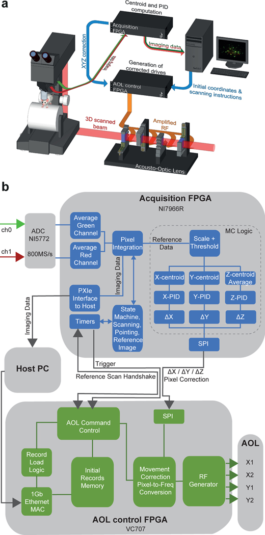
Extended Data Fig. 1
Two-photon microscope and real time 3D movement correction system
a: Schematic diagram of acousto-optic lens (AOL)nmicroscope and FPGA-based closed loop control and acquisition system fornreal time 3D movement correction (RT-3DMC). Scanning instructions are sentnfro...
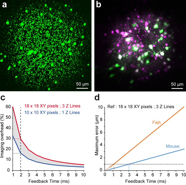
Extended Data Fig. 2
Real time 3D movement correction performance and AOL microscope field of view
a: Example of 1- and 5-u03bcm fluorescent beadsndistributed in agarose in a 400u00d7400 u03bcm FOV using the maximumnscan angle for the AOL with an Olympus XLUMPlanFLN 20X objective lens. Fallnoff in ...
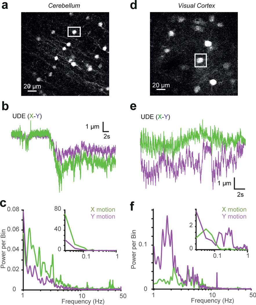
Extended Data Fig. 3
Characterisation of XY movement and frequency spectrum of brain movement
a: Image of cerebellar molecular layer interneuronsnexpressing GFP used to determine brain movement. The white square shows thenselected soma that was used as a reference. b: X (green) and Y (purple) ...
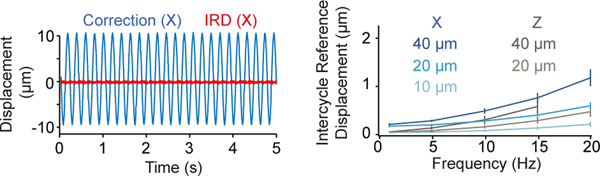
Extended Data Fig. 4
Performance of real time 3D movement correction with a 0.8 NA 40X objective
Left: Tracking of a 1-u03bcm diameter bead on anpiezoelectric stage driven with a sinusoidal drive at 5 Hz. The absolutenreference bead displacement (blue) and the Intercycle Reference Displacementn(I...
Extended Data Fig. 5
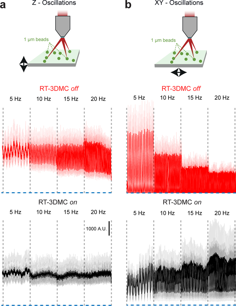
Performance of real-time 3D movement correction for 3D random access point measurements
a: Top: Schematic diagram of imaging 1-u03bcm fluorescentnbeads embedded in agarose, mounted on a piezoelectric driven microscopenstage oscillating at 5 to 20 Hz in the axial direction. Bottom: Random...
Extended Data Fig. 6
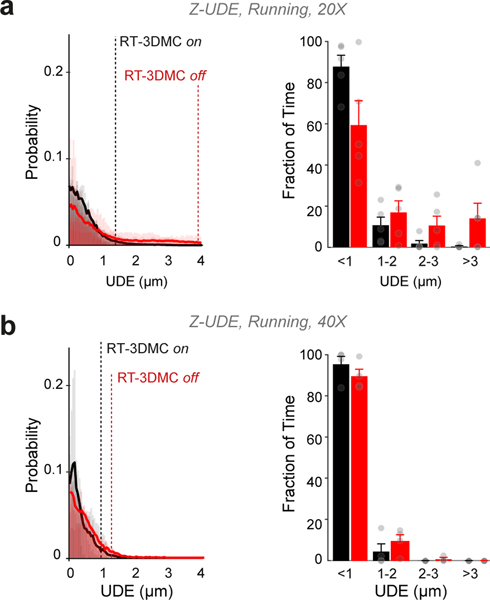
Axial correction of movement with 20X and 40X objective lenses
a: Using a 20X lens: Left :nDistribution of residual Z displacement as estimated by tracking the centernof the cell with RT-3DMC on (black) or off (red) and mean residual movement during periods of lo...
Extended Data Fig. 7
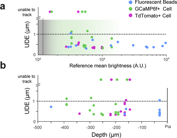
Comparison of beads and somas as reference objects
a: Comparison of tracking performance for differentnfluorescence reference objects with different intensities during locomotionn(20X objective, n=4 mice); 4-u03bcm, red fluorescent beads (blue),nactiv...
Extended Data Fig. 8
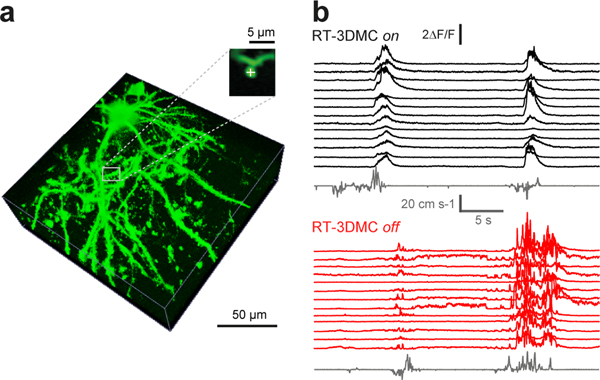
Example of 3D random access point measurement from spines
a: Example of high contrast 3D projection of layer 2/3npyramidal cell and image of a single selected spine (n = 1). b: An example of u0394F/F traces from random accessnpoint measurement from 13 spines...
Extended Data Fig. 9
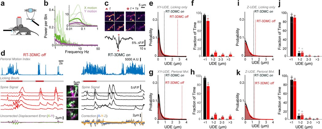
Brain movement and real time 3D movement correction during licking and perioral movements
a: Cartoon of head fixed mouse and arrangement of waternspout. b: Power spectrum of X (green) and Y (purple) motion ofnthe motor cortex during licking bouts. Green and purple thin lines show thenavera...
Extended Data Fig. 10
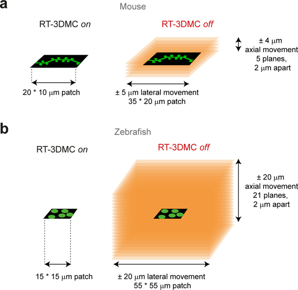
Speed improvements with real-time 3D movement correction
Schematic diagrams comparing the size of patch versus subvolumenneeded to keep the ROIs in the imaging frame with RT-3DMCn( left ) and without RT-3DMCn( right ): a: Imaging dendrites in a mouse with a...
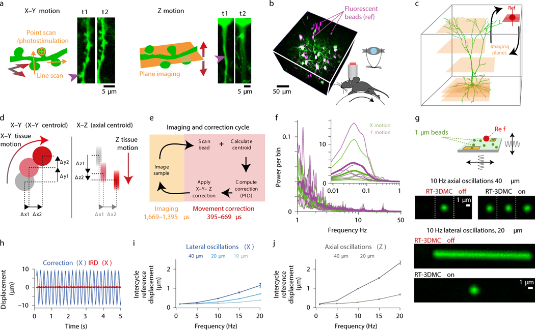
Figure 1:
Design and performance of the real-time 3D movement correction system.
a : Schematic of dendrite and fluorescence images at twontimepoints (t1, t2) illustrating effect of lateral ( left ) andnaxial ( right ) brain motion. Purple arrows indicate lostnfeatures. b: Z-stack ...
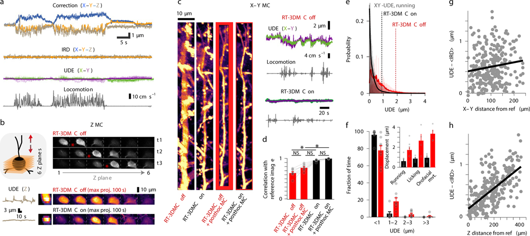
Figure 2:
Monitoring and compensating for brain movement in behaving mice.
a: Top : Example of displacement estimated by tracking a bead innmotor cortex during locomotion (X, blue; Y orange, Z, brown). Center: IRD after RT-3DMC and X and Y UDE (green andnpurple) from 9 patch...
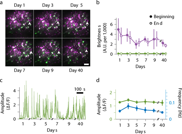
Figure 3:
Longitudinal imaging using real-time 3D movement correction
a: Example of maximum intensity projections of Z stacksnfrom the motor cortex expressing GCaMP6f (green) and tdTomato (magenta) aftern> 1 hour imaging sessions of the same region every other day for 9...
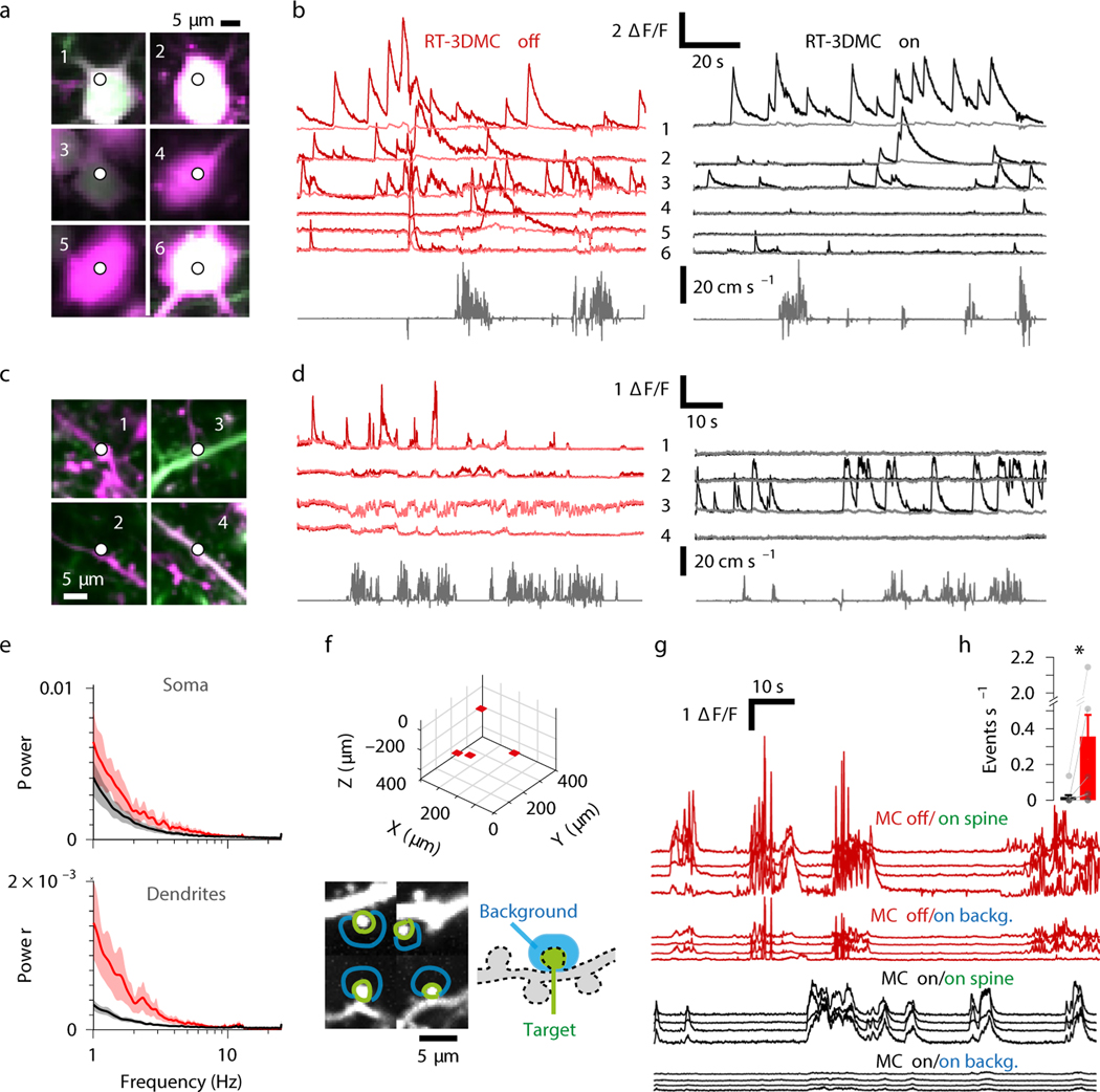
Figure 4:
High-speed recordings of somatic, dendritic and spine activity during locomotion.
a: Location of 3D random access point measurementsn(3D-RAP) on six selected pyramidal cell somata expressing GCaMP6f (green) andntdTomato (magenta) in the motor cortex. b: Example of 3D-RAP measuremen...
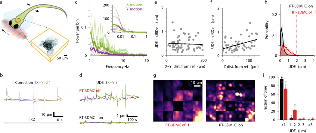
Figure 5:
Monitoring and compensating for brain movement in partially tethered larval zebrafish.
a: Cartoon of zebrafish larva with the rostral bodynsection embedded in agarose (light blue). Inset shows a RT-3DMC Z-stack image ofnthe forebrain expressing nuclear-localized GCaMP6s within the imagi...
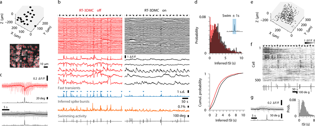
Figure 6:
Functional imaging in behaving zebrafish larvae.
a: Location of 20 imaging patches distributed within thenvolume ( top ), image of 90 neurons monitored for functionalnimaging ( bottom ). b: Nuclear-localised GCaMP6s activity extracted fromnpatches o...
Figure images are served from the NIH/NLM PubMed Central Open Access Subset or Europe PMC; copyright remains with the publishers and authors.
💬 Discussion
0 commentsNo comments yet. Be the first to start a discussion!
Leave a Comment