Abstract
AbstractA fundamental challenge in fluorescence microscopy is the photon shot noise arising from the inevitable stochasticity of photon detection. Noise increases measurement uncertainty and limits imaging resolution, speed and sensitivity. To achieve high-sensitivity fluorescence imaging beyond the shot-noise limit, we present DeepCAD-RT, a self-supervised deep learning method for real-time noise suppression. Based on our previous framework DeepCAD, we reduced the number of network parameters by 94%, memory consumption by 27-fold and processing time by a factor of 20, allowing real-time processing on a two-photon microscope. A high imaging signal-to-noise ratio can be acquired with tenfold fewer photons than in standard imaging approaches. We demonstrate the utility of DeepCAD-RT in a series of photon-limited experiments, including in vivo calcium imaging of mice, zebrafish larva and fruit flies, recording of three-dimensional (3D) migration of neutrophils after acute brain injury and imaging of 3D dynamics of cortical ATP release. DeepCAD-RT will facilitate the morphological and functional interrogation of biological dynamics with a minimal photon budget.
🔬 Techniques
🔭 Microscopes
🧬 Organisms
💻 Software
✨ Fluorophores
🧪 Sample Preparation
🔬 Cell Lines
🏭 Microscope Brands
🧪 Reagent Suppliers
🔴 Lasers
📷 Detectors
🎨 Filters
💻 Software Details
💾 Data Repositories
🏛️ Research Organizations (ROR)
Affiliated research institutions:
📋 Methods
Imaging system
The optical setup integrated two two-photon microscopes for different purposes. One was a standard two-photon microscope with multicolor detection capabilities for multilabeling imaging and cross-system validation. The other was a custom-designed two-photon microscope to capture synchronized low-SNR and high-SNR (tenfold fluorescence photons) images for result validation (Extended Data Fig. 4 ). The two systems shared a titanium-sapphire femtosecond laser source with tunable wavelength (Mai Tai HP, Spectra-Physics). The excitation laser for all experiments was a linearly polarized Gaussian beam with a 920-nm central wavelength and an 80-MHz repetition rate. Before being projected into both systems, the laser beam was first adjusted in polarization by a half-wave plate (AQWP10M-980, Thorlabs) and modulated in intensity by an electro-optic modulator (350-80LA-02, Conoptics). A 1:1 4f system composed of two achromatic convex lenses (AC508-100-B, Thorlabs) was then configured to collimate the laser beam. Another 1:4 4f system (AC508-100-B and AC508-400-B, Thorlabs) was followed to expand the diameter of the beam. A mirror mounted on a two-position, motorized flip mount (MFF101, Thorlabs) was used to alternate between the two systems (OFF for the multicolor module and ON for the custom module). The two systems used the same optical configuration for two-photon excitation. Specifically, the collimated, scaled laser beam was successively guided onto the fast axis (the resonant mirror) and the slow axis (the galvanometric mirror) of the galvo-resonant scanner (8315K/CRS8K, Cambridge Technology). The scanner provided fast 2D raster scanning under the control of two voltage signals. The orientation of the incident beam should be fine-adjusted to ensure the horizontality of the outgoing beam. Then, the output beam was recollimated, rescaled and corrected by a scan lens (SL50-2P2, Thorlabs) and a tube lens (TTL200MP, Thorlabs) to fit the back pupil of the objective and produce a flat image plane. We used a high numerical aperture (NA) water-immersion objective (×25/1.05-NA, XLPLN25XWMP2, Olympus) to expand the detection angle and increase the number of photons that can be detected. Approximately, the effective excitation NA was 0.7 in our experiments. To perform 3D volumetric imaging, we mounted the objective on a piezoelectric actuator (P-725, Physik Instrumente) to achieve high-precision axial scanning. For the detection path of the standard multicolor system, fluorescence photons emitted from the sample were captured by the objective and separated from the excitation light by a long-pass dichroic mirror (DMLP650L, Thorlabs). Another short-pass dichroic mirror (DMSP550, Thorlabs) was mounted in the detection path to separate green fluorescence and red fluorescence. The green fluorescence was purified by a pair of emission filters (MF525-39, Thorlabs; ET510/80M, Chroma) and detected by a GaAsP photomultiplier tube (PMT; H10770PA-40, Hamamatsu). The red fluorescence was filtered by an emission filter (ET585/65M, Chroma) and detected by the same type of PMT. For the detection path of the customized system for simultaneous low-SNR and high-SNR imaging, the previously mentioned short-pass dichroic mirror was replaced with a 1:9 (reflectance:transmission) non-polarizing plate beam splitter (BSN10, Thorlabs). Low-SNR images were formed by the ~10% reflected photons, and high-SNR images were formed by the ~90% transmitted photons. In this system, only green fluorescence was detected, and the same filters and PMT were used for both the low-SNR and high-SNR detection paths. The sensor plane of each PMT was conjugated to the back pupil plane of the objective using a 4:1 4f system (TTL200-A and AC254-050-A, Thorlabs) to maximize the detection efficiency. In general, the maximum FOV of the two two-photon microscopes was about 720 μm. The typical frame rate was 30 Hz for 512 × 512 pixels, and the volume rate decreased linearly with the number of planes to be scanned.
Show full methods section
Imaging system
The optical setup integrated two two-photon microscopes for different purposes. One was a standard two-photon microscope with multicolor detection capabilities for multilabeling imaging and cross-system validation. The other was a custom-designed two-photon microscope to capture synchronized low-SNR and high-SNR (tenfold fluorescence photons) images for result validation (Extended Data Fig. 4 ). The two systems shared a titanium-sapphire femtosecond laser source with tunable wavelength (Mai Tai HP, Spectra-Physics). The excitation laser for all experiments was a linearly polarized Gaussian beam with a 920-nm central wavelength and an 80-MHz repetition rate. Before being projected into both systems, the laser beam was first adjusted in polarization by a half-wave plate (AQWP10M-980, Thorlabs) and modulated in intensity by an electro-optic modulator (350-80LA-02, Conoptics). A 1:1 4f system composed of two achromatic convex lenses (AC508-100-B, Thorlabs) was then configured to collimate the laser beam. Another 1:4 4f system (AC508-100-B and AC508-400-B, Thorlabs) was followed to expand the diameter of the beam. A mirror mounted on a two-position, motorized flip mount (MFF101, Thorlabs) was used to alternate between the two systems (OFF for the multicolor module and ON for the custom module). The two systems used the same optical configuration for two-photon excitation. Specifically, the collimated, scaled laser beam was successively guided onto the fast axis (the resonant mirror) and the slow axis (the galvanometric mirror) of the galvo-resonant scanner (8315K/CRS8K, Cambridge Technology). The scanner provided fast 2D raster scanning under the control of two voltage signals. The orientation of the incident beam should be fine-adjusted to ensure the horizontality of the outgoing beam. Then, the output beam was recollimated, rescaled and corrected by a scan lens (SL50-2P2, Thorlabs) and a tube lens (TTL200MP, Thorlabs) to fit the back pupil of the objective and produce a flat image plane. We used a high numerical aperture (NA) water-immersion objective (×25/1.05-NA, XLPLN25XWMP2, Olympus) to expand the detection angle and increase the number of photons that can be detected. Approximately, the effective excitation NA was 0.7 in our experiments. To perform 3D volumetric imaging, we mounted the objective on a piezoelectric actuator (P-725, Physik Instrumente) to achieve high-precision axial scanning. For the detection path of the standard multicolor system, fluorescence photons emitted from the sample were captured by the objective and separated from the excitation light by a long-pass dichroic mirror (DMLP650L, Thorlabs). Another short-pass dichroic mirror (DMSP550, Thorlabs) was mounted in the detection path to separate green fluorescence and red fluorescence. The green fluorescence was purified by a pair of emission filters (MF525-39, Thorlabs; ET510/80M, Chroma) and detected by a GaAsP photomultiplier tube (PMT; H10770PA-40, Hamamatsu). The red fluorescence was filtered by an emission filter (ET585/65M, Chroma) and detected by the same type of PMT. For the detection path of the customized system for simultaneous low-SNR and high-SNR imaging, the previously mentioned short-pass dichroic mirror was replaced with a 1:9 (reflectance:transmission) non-polarizing plate beam splitter (BSN10, Thorlabs). Low-SNR images were formed by the ~10% reflected photons, and high-SNR images were formed by the ~90% transmitted photons. In this system, only green fluorescence was detected, and the same filters and PMT were used for both the low-SNR and high-SNR detection paths. The sensor plane of each PMT was conjugated to the back pupil plane of the objective using a 4:1 4f system (TTL200-A and AC254-050-A, Thorlabs) to maximize the detection efficiency. In general, the maximum FOV of the two two-photon microscopes was about 720 μm. The typical frame rate was 30 Hz for 512 × 512 pixels, and the volume rate decreased linearly with the number of planes to be scanned.
System calibration
We imaged green-fluorescent beads to calibrate our imaging systems. For sample preparation, the original bead suspension was first diluted and embedded in 1.0% agarose and mounted on microscope slides to form a single bead layer composed of sparsely distributed beads. We calibrated both systems using 0.2-μm fluorescent beads (G200, Thermo Fisher) to obtain the lateral and axial resolution. Because the two systems had identical excitation optics, they had the same optical resolution. The lateral full width at half maximum (FWHM) is ~0.6 μm, and the axial FWHM is ~3.5 μm (Supplementary Fig. 7 ). To calibrate the intensity ratio between the high-SNR detection path and the low-SNR detection path, we imaged 1-μm fluorescent beads (G0100, Thermo Fisher) and found that the intensity ratio is about 1:10 (Extended Data Fig. 5a–d ), which indicated that the number of fluorescence photons of the high-SNR detection path was about ten times higher than that of the low-SNR detection path. High-SNR data synchronized with low-SNR data could serve as a reference to unveil underlying signals. We also imaged insect slices for validation, and the results confirmed our calibration (Extended Data Fig. 5e–h ). Model simplification Theoretically, large models with more trainable parameters can implement extremely intricate functions on the input data. However, the very big model (16,315,585 (abbreviated 16.3 million) parameters in total) we previously used caused a series of problems, such as long training and inference time, large memory consumption and serious overfitting. We sought to solve these problems by simplifying the network architecture. Because network depth is of crucial importance for the performance 69 , instead of changing the depth of the network, we turned to reduce the number of feature maps in each convolutional layer. By continuously halving network parameters, we constructed seven models with exponentially decreased trainable parameters (16.3 million, 9.2 million, 4.1 million, 2.3 million, 1.0 million, 0.57 million and 0.26 million, respectively). To evaluate these models, we used synthetic calcium imaging data of −2.5 dB SNR and trained them with the same amount of data (6,000 frames). The best training epoch of each model was determined by monitoring its performance on a validation set. Although the number of trainable parameters was reduced by ~94%, the denoising performance did not degrade because overfitting was suppressed effectively. The over-simplified network will also lead to reduced performance because of insufficient network capacity (Supplementary Fig. 2 ). Thus, using the architecture of 1.0 million trainable parameters is the best choice for practical use. A more comprehensive assessment, including training and inference time, memory consumption and output SNR, is shown in Supplementary Table 1 . The lightweight model with ~1.0 million parameters was chosen as the final architecture. Data augmentation The strategy to eliminate overfitting by drastically reducing trainable parameters only works when there is enough training data. If only a small dataset is available, overfitting still occurs even with very small models 70 . To alleviate the data dependency of our method and further eliminate overfitting, we designed 12-fold data augmentation to generate enough training pairs from a small amount of data (Extended Data Fig. 2 ). Given a low-SNR time-lapse image stack, thousands of 3D training pairs with overlaps will be extracted from the input stack. A training pair includes an input patch and a corresponding target patch. The proportion of temporal overlapping was automatically calculated according to the number of training pairs to be extracted. For each training pair, we first swapped the input and target randomly with a probability of 0.5. Then, we performed six geometric transformations randomly for the training pair, including horizontal flip, vertical flip, left 90° rotation, 180° rotation, right 90° rotation and no transformation. Overall, there were 12 possible forms for each training pair, and they all have the same probability of occurrence, which inflated the training dataset by 12-fold. We investigated the benefit of our data augmentation strategy using synthetic calcium imaging data and found that the data dependency of our method was reduced effectively (Supplementary Fig. 3 ). A 1,000-frame calcium imaging stack (490 × 490 pixels) is enough to train a model with satisfactory performance. This feature is helpful to alleviate the problem of insufficient training data in fluorescence microscopy. To evaluate the effect of data augmentation on overfitting, we trained one model with data augmentation and another model without data augmentation with the same amount of data for a long training period (35 epochs) and monitored performance after each epoch. The results showed that training with data augmentation could keep the performance stable compared to the rapidly degrading performance without augmentation (Extended Data Fig. 3 ). The optimal performance was also improved because of augmented training data. Although the combination of model simplification and data augmentation eliminates overfitting, preparing more training data is still the most effective way to improve the denoising performance and avoid overfitting. Network architecture, training and inference The network architecture in this research reserves the topology of 3D U-Net 71 that uses the encoder–decoder architecture in an end-to-end manner. To fully exploit spatiotemporal correlations in fluorescence imaging data, all operations inside the network were implemented in 3D, including convolution, max pooling and interpolation (Extended Data Fig. 8 ). Compared to our previous architecture 33 , the number of feature maps in each convolutional layer was reduced by fourfold, and the total number of trainable parameters was reduced by 16-fold (1,020,337 compared to 16,315,585), which massively improved the training and inference speed and reduced the memory consumption. For preprocessing, each input stack was subtracted by the average of the whole stack to handle the intensity variation across different samples and imaging platforms. These stacks were partitioned into a specified number of 3D ( x - y - t ) training pairs. The data augmentation strategy mentioned above would be applied to each training pair. Training was performed using the arithmetic average of an L1-norm loss term and an L2-norm loss term as the loss function. After the input stack flowed through the network, the subtracted average value would be added back after processing. Because the combination of model simplification and data augmentation eliminated overfitting, the model of the last training epoch could be directly selected as the final solution. For denoising of 3D volumetric imaging, the time-lapse stack of each imaging plane was saved as a separate TIFF file. All stacks were used for the training of the network. The batch size for all experiments was set to the number of GPUs being used. The patch size was set to 150 × 150 × 150 pixels by default. All models were trained using the Adam optimizer 72 with a learning rate of 5 × 10 −5 , and the exponential decay rates for the first-moment and second-moment estimates were 0.5 and 0.9, respectively. Using our Python code, training with 3,000 pairs of 3D patches for 20 epochs took just 6.2 h on a single GPU (GeForce RTX 3090, Nvidia). The inference process for an image stack composed of 490 × 490 × 300 pixels (partitioned into 75 3D patches) took as few as 8 s. Multi-GPU acceleration has been supported by our Python code. The time consumption of training and inference decreases linearly as the number of GPUs increases. Real-time implementation of DeepCAD-RT To achieve real-time processing during imaging acquisition, we made a program interface to incorporate DeepCAD-RT into our image acquisition software (Scanimage 5.7 (ref. 73 ), Vidrio Technologies). For further acceleration and memory conservation, the inference of DeepCAD-RT was optimally deployed on GPU with TensorRT (Nvidia), a software development kit providing low-latency and high-throughput processing for deep learning applications by executing customized operation automatically for specific GPU and network architecture. Three parallel threads were designed for imaging, data processing and display. The schedule for multithread programming is depicted in Fig. 1c . Specifically, the first thread was used for image acquisition, which waited for a certain number of frames and packaged them into 3D ( x - y - t ) batches. Adjacent batches had overlapping frames, and half of the overlap would be discarded to avoid artifacts. Then, the second thread got low-SNR images passed by the first thread, processed them and produced denoised frames. Finally, these denoised frames were transferred to the third thread for display. When the imaging process stopped, denoised images would be automatically saved in a user-defined directory. The real-time implementation was programmed in C++ for best hardware interaction and compiled in Matlab (MathWorks), which could be called by any Matlab-based software or script. On a single GPU (GeForce RTX 3090, Nvidia), the real-time implementation achieved more than a 20-fold speed up compared to the original DeepCAD 33 and had an extremely low memory consumption, as few as 701 MB with float16 precision. The real-time implementation of DeepCAD-RT has been packaged as a free plugin with a user-friendly interface (Extended Data Fig. 1 ). To transfer pretrained models, scripts were developed to convert PyTorch models to open neural network exchange (ONNX) models and call TensorRT builder to optimize ONNX models for a target GPU, which produced engine files that can be used by TensorRT. The construction of the engine file would eliminate dead computations, fold constants and combine operations to find an optimal schedule for model execution.
Animal preparation and fluorescence imaging
Multiple animal models (mice, zebrafish and flies) and fluorescence labeling methods (calcium, neutrophils and ATP release) were associated in this research. All experiments involving animals were performed in accordance with the institutional guidelines for animal welfare and have been approved by the Animal Care and Use Committee of Tsinghua University.
Mouse preparation and imaging
Adult mice (male or female without randomization or blinding) at 8–16 postnatal weeks were housed in an animal facility (24 °C and 50% humidity) under a reverse light cycle in groups of one to five. All imaging experiments were performed with our two-photon microscopes on head-fixed, awake mice. For functional imaging of neural activity, we used transgenic mice hybridized between Rasgrf2-2A-dCre mice and Ai148 (TIT2L-GC6f-ICL-tTA2)-D mice expressing Cre-dependent GCaMP6f genetically encoded calcium indicator. Craniotomy surgeries were conducted for chronic two-photon imaging as previously described 33 . Briefly, mice were first anesthetized with 1.5% (by volume in oxygen) isoflurane, and a 6.0-mm-diameter craniotomy was made with a skull drill. After removing the skull piece, a coverslip was implanted on the craniotomy region, and a titanium headpost was then cemented to the skull for head fixation. After the surgery, 0.25 mg per gram (body weight) trimethoprim was injected intraperitoneally to induce the expression of GCaMP6f in layer 2/layer 3 cortical neurons across the whole brain. After inflammation was gone and the cranial window became clear (~2 weeks after surgery), mice were head-fixed on a customized holder with a 3D-printed plastic tube to restrict the mouse body. The holder was mounted on a high-precision, three-axis motorized stage (M-VP-25XA-XYZL, Newport) for sample translation. In vivo calcium imaging (30-Hz single-plane imaging) was performed on awake mice without anesthesia. The imaging of dendritic spines in L1 (20–60 μm below the brain surface) required adequate spatial sampling rate that was achieved by using large zoom factors. For time-lapse imaging of neutrophil migration, we first performed craniotomies on wild-type mice (C57BL/6J) following the procedures described above. Acute brain injury caused by craniotomy induce immune responses in the brain. After surgery, neutrophils and blood vessels were simultaneously labeled by injecting 10 μg of red (Alexa Fluor 555 conjugate) wheat germ agglutinin (WGA) dye ( W32464 , Thermo Fisher Scientific) and 2 μg of green-fluorescence-conjugated Ly-6G/Ly-6C antibody (53-5931-82, eBioscience) intravenously. The two dyes were dissolved and diluted in 200 μl of 1× PBS. To avoid the potential influence of anesthesia on immune responses, in vivo two-photon imaging was performed in the mouse brain after the mouse was fully awake (~20 min after injection). Imaging experiments should be finished as soon as possible because these dyes are degradable in the mouse body. Empirically, the whole imaging session should take no longer than 5 h. Volumetric imaging was implemented by scanning the objective axially with the piezoelectric actuator. The frame rate of single-plane imaging was 30 Hz, and the volume rate of 3D imaging was 2 Hz (15 imaging planes). The whole 3D imaging session lasted ~20 min. For each 3D volume, the flyback frame acquired while the piezoelectric actuator was quickly returning from the bottom plane to the top plane should be discarded. Images of the green channel and the red channel were captured simultaneously and were separated by postprocessing. For functional imaging of ATP dynamics, wild-type mice (C57BL/6J) were anesthetized with intraperitoneally injected Avertin (500 mg per kilogram (body weight), Sigma-Aldrich). A cranial window was opened on the visual cortex, and 400–500 nl of adeno-associated virus (AAV2/9-GfaABC1D-ATP1.0, packaged at Vigene Biosciences) was injected (anterior–posterior: −2.2 mm relative to bregma, medial–lateral: 2.0 mm relative to bregma and dorsal–ventral: 0.5 mm below the dura, at an angle of 30°) using a microsyringe pump (Nanoliter 2000 injector, World Precision Instruments) to express GRAB ATP1.0 (ref. 34 ) in cortical astrocytes. A 4 mm × 4 mm square coverslip was implanted to replace the skull. After ~3 weeks of recovery and virus expression, two-photon imaging was performed to record ATP release events in the mouse cortex. Before imaging, brain injury was induced by ablating the tissue with a stationary laser focus (200 mW) for 5 s. The injury site was located at the center of the 3D imaging volume. Single-plane images were recorded at the plane 20 μm above the injury site. The frame rate of single-plane imaging was 30 Hz, and the volume rate of 3D imaging was 1 Hz (30 imaging planes). The flyback frame of each volume should be discarded. Only signals from the green channel were recorded, and the whole 3D imaging session lasted 60 min.
Zebrafish preparation and imaging
Transgenic zebrafish ( Danio rerio ) larvae expressing pan-neuronal GCaMP6s calcium indicator (Tg(HuC:GCaMP6s)) were housed in culture dishes at 28.5 °C in Holtfreter’s solution (59 mM NaCl, 0.67 mM KCl, 0.76 mM CaCl 2 and 2.4 mM NaHCO 3 ). At 4–6 d after fertilization, zebrafish larvae were separated and restricted in a small drop of 1.0% low-melting-point agarose (Sigma-Aldrich) and mounted on a microscope slide for imaging. A fine-bristle brush was used to adjust the posture of the larvae to keep the dorsal side up before the agarose solidified. After fixation, the larvae were placed under the objective, and Holtfreter’s solution was used as the immersion medium of the objective. Before image acquisition started, we previewed the image and rotated the microscope slide manually to keep the larva horizontal or vertical in the FOV. Two-photon calcium imaging of spontaneous neural activity was performed on the larvae at 26–27 °C without anesthesia or motion paralysis. All experiments were single-plane imaging, and the frame rate was 30 Hz for 512 × 512 pixels. Both large neuronal populations across multiple brain regions and small neuronal subsets localized in the optic tectum were imaged using different zoom factors.
Drosophila preparation and imaging
Flies were raised on standard cornmeal medium with a 12-h light/12-h dark cycle at 25 °C. Transgenic flies UAS-GCaMP7f were crossed with OK107-Gal4 to drive the expression of the GCaMP7f 25 calcium indicator in essentially all Kenyon cells. All experiments were conducted on female F1 heterozygotes from this cross. Flies at 5 d after eclosion were anesthetized on ice and mounted in a 3D-printed plastic disk that allowed free movement of the legs, as previously reported 74 . The posterior head capsule was opened using sharp forceps (5SF, Dumont) at room temperature in carbonated (95% O 2 , 5% CO 2 ) buffer solution (103 mM NaCl, 3 mM KCl, 5mM N-Tris, 10 mM trehalose, 10 mM glucose, 7 mM sucrose, 26 mM NaHCO 3 , 1 mM NaH 2 PO 4 , 1.5 mM CaCl 2 and 4 mM MgCl 2 ) with a pH of 7.3 and an osmolarity of 275 mosM. After that, the air sacks and tracheas were also removed. Brain movement was minimized by adding UV glue around the proboscis and removing the M16 muscle 40 , 75 . After preparation, flies were placed under the objective for two-photon imaging of calcium transients in the mushroom body. To enhance neural activity, 4-methylcyclohexanol and 3-octanol diluted 1:1,000 in mineral oil were used as odors. Flies were randomly given the two odors for 5 s every 10 s using a custom-made air pump. All experiments were single-plane imaging experiments at 30 Hz with 512 × 512 pixels.
Generation of synthetic calcium imaging data
We used synthetic calcium imaging data (simulated time-lapse image sequences) for quantitative evaluations of our method and for comparisons with DeepInterpolation 32 . Our simulation pipeline consisted of synthesizing noise-free calcium imaging videos (ground truth) and adding different levels of mixed Poisson–Gaussian noise 22 , 33 . To generate noise-free calcium imaging data, we adopted in silico NAOMi, a simulation method to create realistic calcium imaging datasets for assessing two-photon microscopy methods 36 . The parameters of our simulation are listed in Supplementary Table 2 . Those not mentioned all used default values. Simulated data had very similar spatiotemporal features to experimentally obtained data, including neuronal anatomy (cell bodies, neuropils, dendrites and so on), neural activity and blood vessels. For noise simulation, we first performed Poisson sampling on noise-free images to simulate the content-dependent Poisson noise. We then added content-independent Gaussian noise to these data. Poisson noise was set as the dominant noise source.
Different imaging
SNRs were simulated by different relative photon numbers that changed the intensity of input noise-free images (Supplementary Fig. 1 ).
Neutrophil segmentation
Four types of data were involved in this experiment, that is, raw data (low-SNR), high-SNR (tenfold fluorescence photons) data, denoised raw data and denoised high-SNR data. Ten representative images with relatively sparse cells were selected from the dataset of single-plane neutrophil imaging for semantic segmentation. To obtain ground-truth segmentation masks, five human experts were recruited to annotate all neutrophils in each denoised high-SNR image using the ROI Manager toolbox of Fiji. The final ground-truth masks were determined by majority voting. Neutrophil segmentation was conducted using Cellpose 46 and Stardist 47 , two CNN-based generalist algorithms for cellular segmentation. For both methods, default parameters and pretrained models were used without additional training. Segmentation performance was quantitatively evaluated with the IoU score 76 defined as documentclass[12pt]{minimal} usepackage{amsmath} usepackage{wasysym} usepackage{amsfonts} usepackage{amssymb} usepackage{amsbsy} usepackage{mathrsfs} usepackage{upgreek} setlength{oddsidemargin}{-69pt} begin{document}$${{{mathrm{IoU}}}} = frac{{{{{mathrm{A}}}} cap {{{mathrm{B}}}}}}{{{{{mathrm{A}}}} cup {{{mathrm{B}}}}}},$$end{document} IoU = A ∩ B A ∪ B , where A is the mask segmented by algorithms and B is the ground truth. Statistical analysis and representative results are summarized in Extended Data Fig. 7 .
Three-dimensional visualization
For volumetric imaging of neutrophil migration and ATP release, we performed 3D visualization to reveal the spatiotemporal patterns of biological dynamics. Imaris 9.0 (Oxford Instruments) was used for the visualization of all volumetric imaging data. Both the original low-SNR data and denoised data were imported into Imaris, rendered with pseudocolor and 3D reconstructed using the maximum intensity projection mode. The brightness of data before and after denoising was adjusted to make them have a similar visual effect. The contrast of low-SNR data was fine-tuned to show underlying signals as clearly as possible. All values for gamma correction were set to one. The red channel (blood vessels) of neutrophil migration was averaged by multiple frames to improve its SNR and merged with the green channel. Cross-talk signals out of the blood vessel were manually suppressed with Fiji. Animations were generated by automatically interpolating intermediate frames between selected keyframes. Annotation of ATP release events The whole annotation pipeline was implemented on the denoised data (Supplementary Fig. 8 ). The spatial shape of each ATP release event could be modeled as an ellipsoid. To obtain the center position and peak time of each event throughout the whole imaging session, we manually annotated them by adding measurement points in Imaris. All spatial and temporal coordinates were exported from the software after annotation. Events at the edge of the volume were excluded because only a part of them appeared in the FOV. Based on these annotated coordinates, intensity profiles along all three dimensions of each event were extracted from denoised stacks with a custom Matlab (MathWorks) script. Gaussian fitting was performed for all intensity profiles to reduce the influence of background fluctuations. All fitted Gaussian curves were then deconvolved with the system point spread function using a standard Richardson–Lucy algorithm 77 , 78 . This step eliminated the influence of limited and anisotropic spatial resolution. The diameter of these ATP release events could be extracted in each dimension, which was defined as the FWHM of deconvolved Gaussian curves. The ellipticity of release events was defined as documentclass[12pt]{minimal} usepackage{amsmath} usepackage{wasysym} usepackage{amsfonts} usepackage{amssymb} usepackage{amsbsy} usepackage{mathrsfs} usepackage{upgreek} setlength{oddsidemargin}{-69pt} begin{document}$${{{mathrm{ellipticity}}}} = frac{{a - b}}{a},$$end{document} ellipticity = a − b a , where a is the major axis of the ellipse, and b is the minor axis of the ellipse. Ellipticity was calculated for each 3D release event in all three orthogonal coordinate planes ( x - y , y - z and x - z ).
Method comparison
Four baseline methods are included in the comparison. Synthetic calcium imaging images (6,000 frames, 30 Hz frame rate) were used for the training and testing of all methods. For each method, a specified model was trained for each SNR level. The supervised baseline was obtained with a larger 3D U-Net (4.1 million trainable parameters) trained in a supervised manner. All hyperparameters were kept the same with DeepCAD-RT. DeepInterpolation was implemented with the companion code of relevant papers 32 , and two kinds of DeepInterpolation models were trained using default hyperparameters. The first model was trained from scratch. The other model was fine-tuned based on a pretrained model (pretrained with 225,000 two-photon images of the Ai93 reporter line) by presenting the training data only once according to the DeepInterpolation paper. Noise2Void 37 models were trained for 50 epochs with 64 × 64 patch size and 128 batch size. HDN is the upgraded version of DivNoising 79 with state-of-the-art performance. Because no calibration data are available, the noise models of HDN were bootstrapped from the noisy data, and the conditional distributions were estimated from paired noisy images and pseudo-ground truth (obtained from Noise2Void). The noise models were trained for 10,000 epochs with a batch size of 250,000 and 0.01 learning rate. The final HDN model of each SNR was trained for 150 epochs, and the best training epoch was selected by evaluating the output SNR of the first 10 frames. The minimum mean square error estimate of each frame was obtained by averaging 100 denoised samples. All hyperparameters not mentioned here were set as default values.
Performance metrics
To quantitatively evaluate the performance of our method, both synthetic data and experimentally obtained data were used. For synthetic calcium imaging data, ground-truth images were available, and SNR was calculated to quantify the denoising performance. SNR was defined as the logarithmic form documentclass[12pt]{minimal} usepackage{amsmath} usepackage{wasysym} usepackage{amsfonts} usepackage{amssymb} usepackage{amsbsy} usepackage{mathrsfs} usepackage{upgreek} setlength{oddsidemargin}{-69pt} begin{document}$${mathrm{SNR}} = 10 cdot log _{10}frac{{left| y right|_2^2}}{{left| {x - y} right|_2^2}},$$end{document} SNR = 10 ⋅ log 10 y 2 2 x − y 2 2 , where x is the denoised data, and y is the ground truth. For experimentally obtained data, synchronized high-SNR data with tenfold photons acquired with our system were used as the reference of underlying signals. Pearson correlation coefficient ( R ) was used as the performance metric, which is formulated as documentclass[12pt]{minimal} usepackage{amsmath} usepackage{wasysym} usepackage{amsfonts} usepackage{amssymb} usepackage{amsbsy} usepackage{mathrsfs} usepackage{upgreek} setlength{oddsidemargin}{-69pt} begin{document}$$R = frac{{{{{mathrm{E}}}}left[ {(x - mu _x)(y - mu _y)} right]}}{{sigma _xsigma _y}},$$end{document} R = E ( x − μ x ) ( y − μ y ) σ x σ y , where x and y are the denoised data and corresponding high-SNR data, respectively; μ x and μ y are the mean values of x and y ; and σ x and σ y are the standard deviations. The operator E represents arithmetically averaging. Pearson correlation was used for both images and fluorescence traces. All performance metrics were implemented with custom Matlab scripts and built-in functions.
Statistics and reproducibility
Sample sizes and statistics are reported in the figure legends and text for each experiment. All box plots were plotted in the format of standard Tukey box and whisker plots. The box indicates the lower and upper quartiles, while the line in the box shows the median. The lower whisker represents the first data point greater than the lower quartile minus 1.5× the interquartile range. Similarly, the upper whisker represents the last data point less than the upper quartile plus 1.5× the interquartile range. Outliers were plotted in small black dots. For the comparison of images and fluorescence traces before and after denoising, a one-sided paired t -test was performed, and P values are indicated with asterisks. Representative frames were demonstrated in the figures, and similar results were achieved on more than 1,500 frames for all experiments. Reporting summary Further information on research design is available in the Nature Research Reporting Summary linked to this article.
Method comparison
Four baseline methods are included in the comparison. Synthetic calcium imaging images (6,000 frames, 30 Hz frame rate) were used for the training and testing of all methods. For each method, a specified model was trained for each SNR level. The supervised baseline was obtained with a larger 3D U-Net (4.1 million trainable parameters) trained in a supervised manner. All hyperparameters were kept the same with DeepCAD-RT. DeepInterpolation was implemented with the companion code of relevant papers 32 , and two kinds of DeepInterpolation models were trained using default hyperparameters. The first model was trained from scratch. The other model was fine-tuned based on a pretrained model (pretrained with 225,000 two-photon images of the Ai93 reporter line) by presenting the training data only once according to the DeepInterpolation paper. Noise2Void 37 models were trained for 50 epochs with 64 × 64 patch size and 128 batch size. HDN is the upgraded version of DivNoising 79 with state-of-the-art performance. Because no calibration data are available, the noise models of HDN were bootstrapped from the noisy data, and the conditional distributions were estimated from paired noisy images and pseudo-ground truth (obtained from Noise2Void). The noise models were trained for 10,000 epochs with a batch size of 250,000 and 0.01 learning rate. The final HDN model of each SNR was trained for 150 epochs, and the best training epoch was selected by evaluating the output SNR of the first 10 frames. The minimum mean square error estimate of each frame was obtained by averaging 100 denoised samples. All hyperparameters not mentioned here were set as default values.
Online content Any methods, additional references, Nature Research reporting summaries, source data, extended data, supplementary information, acknowledgements, peer review information; details of author contributions and competing interests; and statements of data and code availability are available at 10.1038/s41587-022-01450-8.
Supplementary information Supplementary Information Supplementary Figs. 1–8 and Tables 1 and 2. Reporting Summary Supplementary Video 1 Demonstrating real-time denoising on a two-photon microscope using DeepCAD-RT. Supplementary Video 2 DeepCAD-RT enhances the in vivo recording of calcium transients in dendritic spines. Supplementary Video 3 DeepCAD-RT massively improves the imaging SNR of neuronal population recordings in the zebrafish brain. Supplementary Video 4 DeepCAD-RT massively improves the imaging SNR of neuronal population recordings across multiple brain regions in the zebrafish brain. Supplementary Video 5 DeepCAD-RT enhances neuronal population imaging of Drosophila mushroom bodies. Supplementary Video 6 Denoising performance of DeepCAD-RT on two-photon imaging of neutrophils in the mouse brain. Supplementary Video 7 DeepCAD-RT facilitates high-SNR observations of retraction fiber dynamics during neutrophil migration. Supplementary Video 8 DeepCAD-RT reveals the 3D migration of neutrophils in vivo after acute brain injury. Supplementary Video 9 Denoising performance of DeepCAD-RT on a recently developed genetically encoded ATP sensor. Supplementary Video 10 DeepCAD-RT reveals the ATP dynamics of astrocytes in 3D after laser-induced brain injury.
Supplementary information The online version contains supplementary material available at 10.1038/s41587-022-01450-8.
📊 Figures
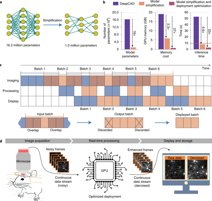
Fig. 1
Optimization and real-time schedule of DeepCAD-RT.
a , Model simplification by feature pruning. The total number of model parameters was reduced from ~16.3 million (16,315,585) to ~1.0 million (1,020,337) for higher processing speed and less memory co...
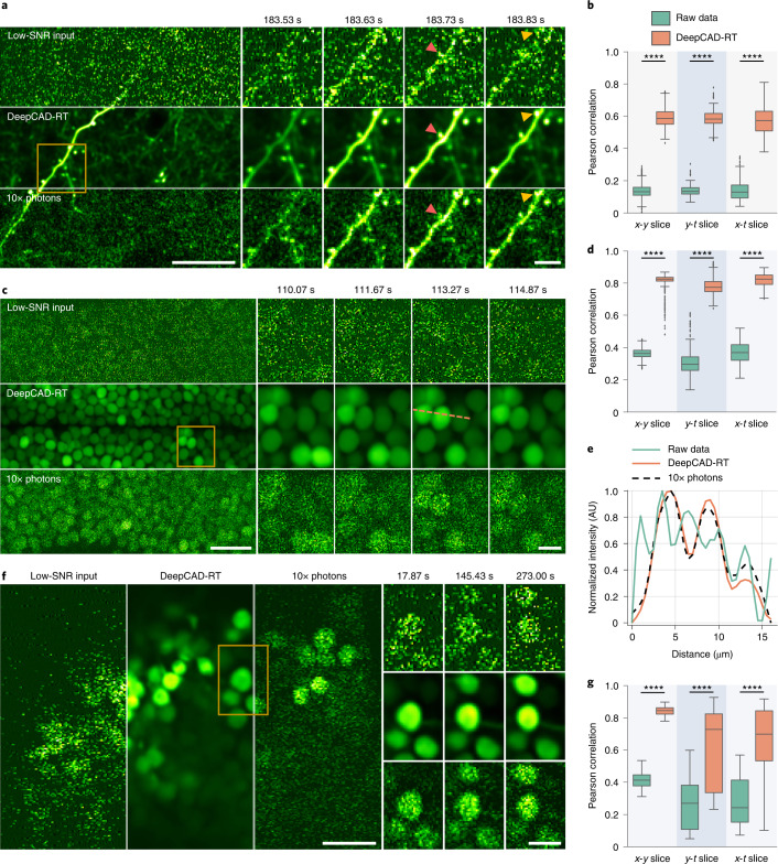
Fig. 2
Universal denoising of calcium imaging in mice, zebrafish and Drosophila .
a , Imaging calcium transients in dendritic spines of a mouse expressing genetically encoded GCaMP6f calcium indicator. One example frame is shown for the low-SNR raw recording (top), DeepCAD-RT denoi...
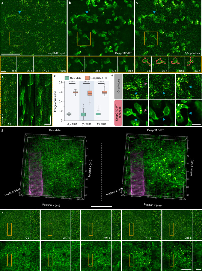
Fig. 3
Observing 3D migration of neutrophils in the mouse brain in vivo.
a , Low-SNR images of neutrophil migration without denoising. b , Images denoised with DeepCAD-RT. c , Synchronized high-SNR images with tenfold fluorescence photons. Blue arrowheads point to the elon...
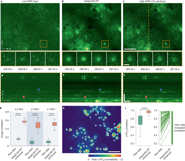
Fig. 4
Denoising performance of DeepCAD-RT on neurotransmitter imaging in live mice.
a , Low-SNR recording of extracellular ATP release in the mouse brain. b , DeepCAD-RT enhanced data with low-SNR recording as the input. c , Synchronized high-SNR data with tenfold photons. Magnified ...
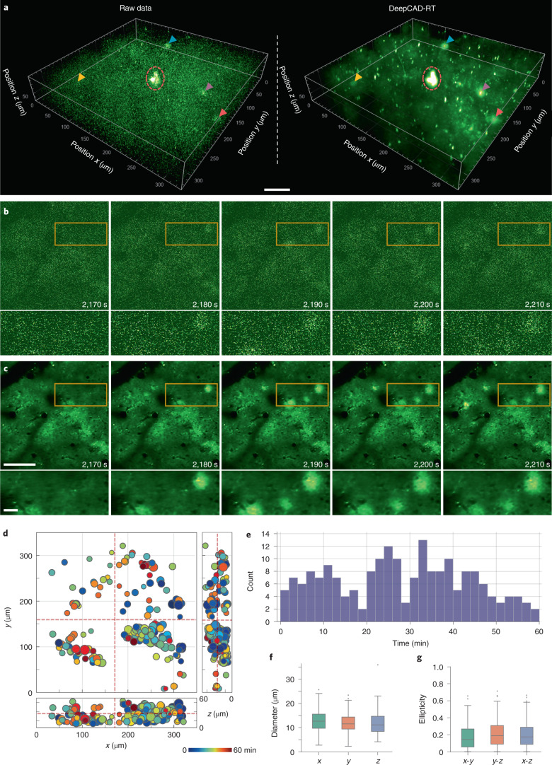
Fig. 5
DeepCAD-RT reveals the spatiotemporal patterns of extracellular ATP in vivo after laser-induced brain injury.
a , Three-dimensional visualization of ATP release events in a 350u2009u00d7u2009350u2009u00d7u200960u2009u03bcm 3 volume (30 planes, 1-Hz volume rate) after laser-induced brain injury. Left, low-SNR ...
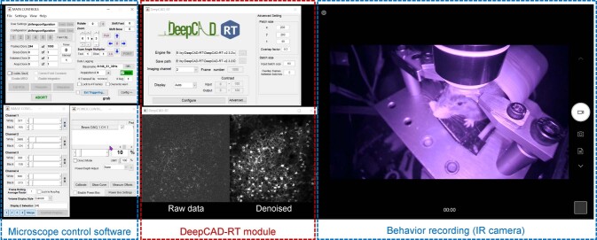
Extended Data Fig. 1
Real-time implementation of DeepCAD-RT.
Real-time denoising was implemented by incorporating DeepCAD-RT into the image acquisition software. Images captured by the microscope were seamlessly fed into DeepCAD-RT, which denoised the input low...
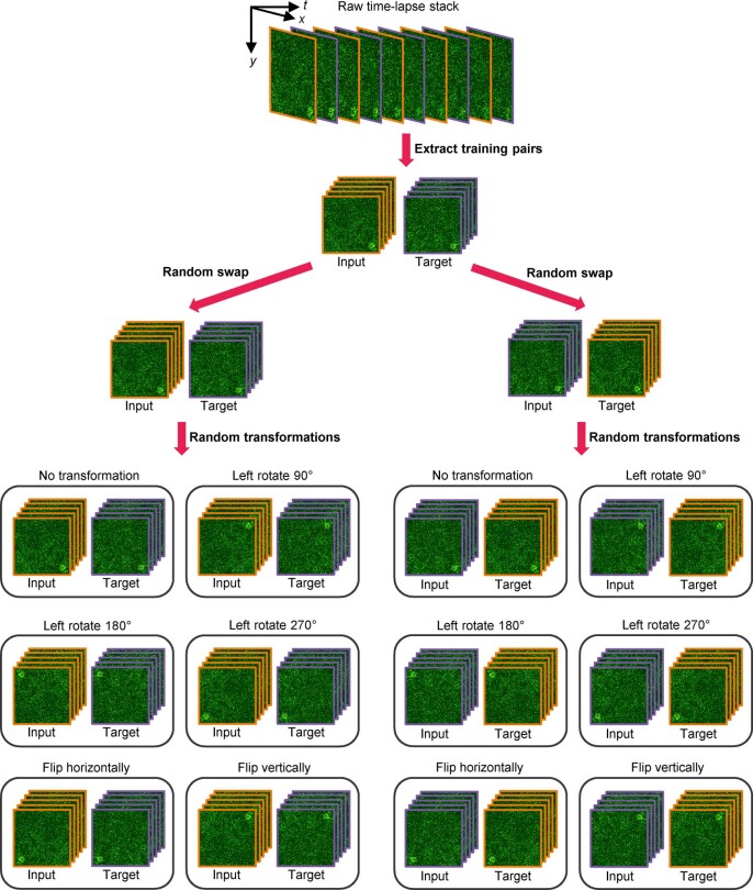
Extended Data Fig. 2
Data augmentation strategy.
Adjacent frames in the original low-SNR stack (xy-t) were divided into two sub-stacks. One as the input volume and the other one as the target volume. Before being fed into the network for training, e...
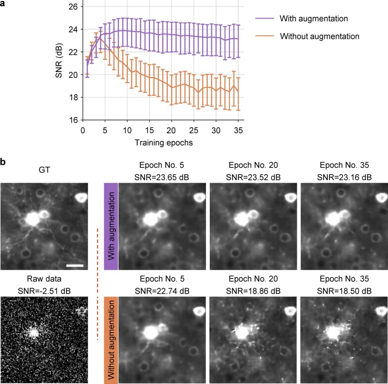
Extended Data Fig. 3
Training stability with and without data augmentation method.
Simulated data (1000 frames, 30u2009Hz frame rate, SNRu2009=u2009u22122.51u2009dB) were used in this experiment for quantitative evaluation. The network architecture has been simplified (~1.0 million ...
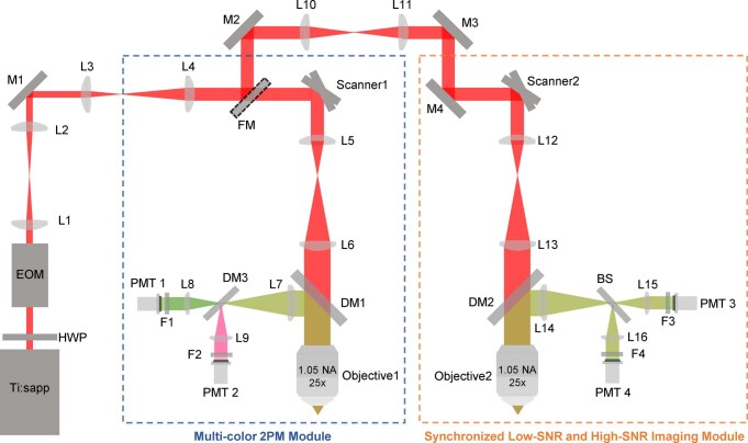
Extended Data Fig. 4
Imaging system.
Our imaging system was composed of a multi-color two-photon module (blue box) and a custom-designed two-photon module to capture synchronized low-SNR and high-SNR images (yellow box). Ti:sapp: titaniu...
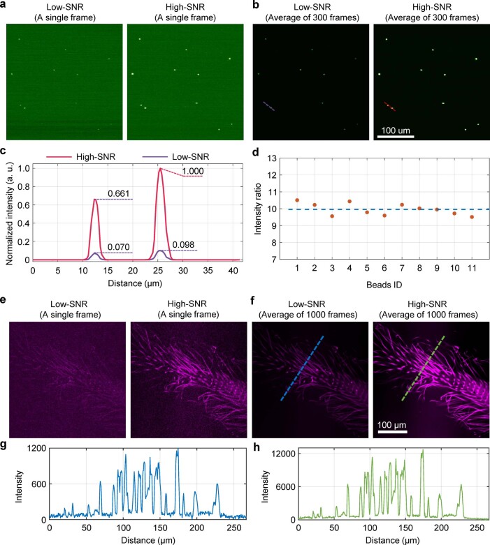
Extended Data Fig. 5
System calibration.
a , Example frames captured by the low-SNR detection path (left) and the high-SNR detection path (right). b , Average projection of 300 continuously acquired frames. Noise was largely suppressed and u...
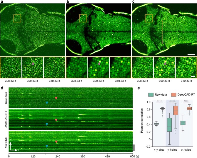
Extended Data Fig. 6
Denoising calcium imaging across multiple brain regions in larval zebrafish.
a , Original low-SNR recording. b , DeepCAD-RT enhanced data. c , Synchronous high-SNR recording with 10-fold fluorescence photons. Magnified views of the yellow boxed region showing calcium dynamics ...
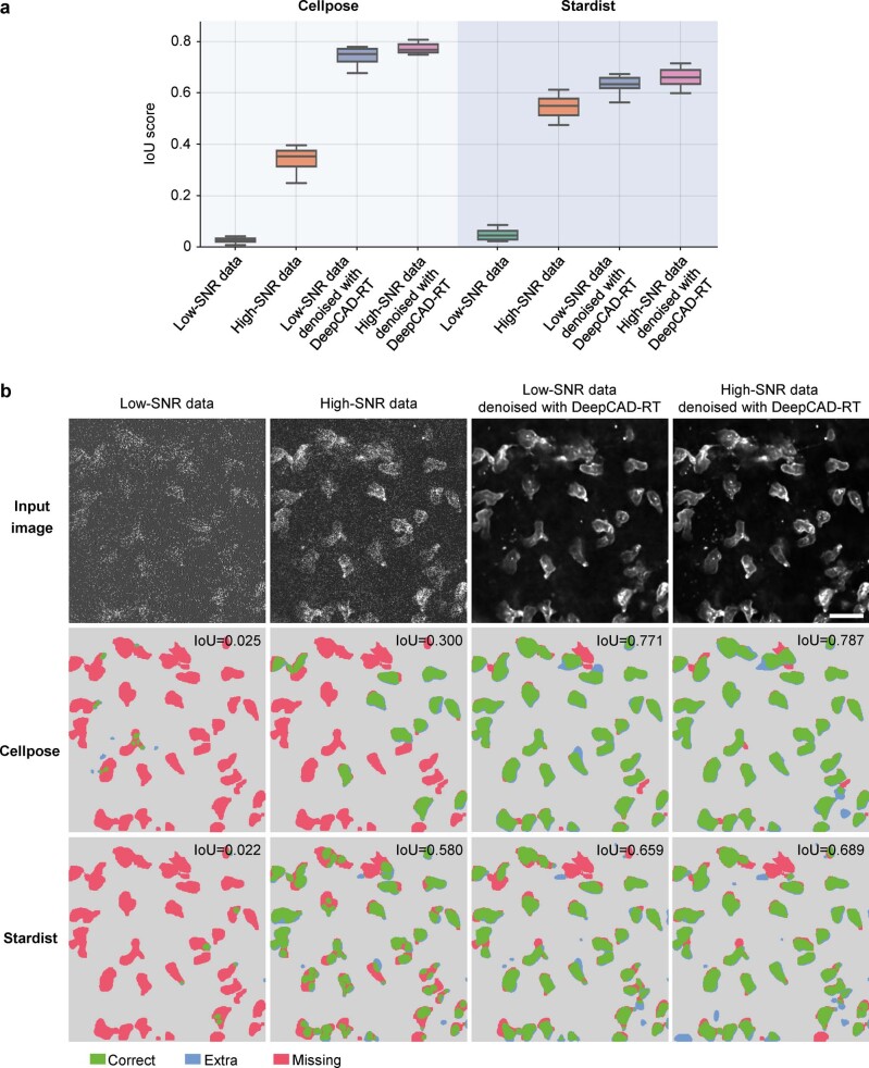
Extended Data Fig. 7
The performance of neutrophil segmentation before and after denoising.
a , Segmentation performance of Cellpose 46 and Stardist 47 on raw low-SNR data, synchronous high-SNR data (10-fold fluorescence photons), DeepCAD denoised raw data, and DeepCAD denoised high-SNR data...
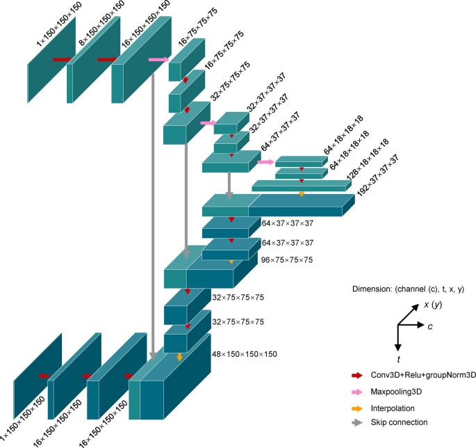
Extended Data Fig. 8
Network architecture.
We used simplified 3D U-net 71 as the network architecture, which is composed of a 3D encoder module, a 3D decoder module, and skip connections from the encoder module to the decoder module. The netwo...
Figure images are served from the NIH/NLM PubMed Central Open Access Subset or Europe PMC; copyright remains with the publishers and authors.
💬 Discussion
0 commentsNo comments yet. Be the first to start a discussion!
Leave a Comment